 2017, Vol. 32


重、磁方法具有成本低、周期短、覆盖面广等特点,已成为解决空间探测、大地构造、区域构造,固体矿产勘探、能源勘探、地震及地质灾害预测、环境及工程检测等方面问题不可或缺的重要手段.目前,位场数据处理和转换分别在空间域和频率域中进行,频率域中的位场数据处理和转换主要是基于Fourier变换(侯重初和刘秀芳,1978;Nagendra R, 1984;吴宣志等,1987;朱文孝等,1989;穆石敏等,1990)、余弦变换(张凤旭等, 2006, 2007)、Hilbert变换(Nabighian,1972;Stanley and Green, 1976;Mohan et al., 1982;张凤旭等,2005;骆遥等,2011)、小波变换(李宗杰等,1997;Li and Oldenburg, 1998)以及Hartley变换(Rao et al., 1996;魏雅利和骆遥,2010;骆遥,2013;马国庆等,2014)来实现的.由于频率域位场数据处理和转换有计算公式简单、计算效率高的特点,是位场数据处理和转换的研究重点.Hartley变换是电气工程师Hartley(1942)提出的一种类似于Fourier变换的实数域积分变换方法.著名的Fourier分析专家Bracewell(1983)首次提出了离散Hartley变换(DHT)的定义.随后不少学者(Bracewell,1984;Hou,1987)提出了Hartley变换的快速算法(FHT).理论上,DHT所需的内存和计算时间要比复数域DFT(离散Fourier变换)节省近一半(Bracewell,1986),已有部分关于Hartley变换研究及应用的文章发表在IEEE所属期刊上,其广泛应用及显示出的重要作用也为地球物理学家所重视.自1990年开始,Saatcilar等(1990)最早将Hartley变换引入到地球物理领域.同年,Marobhe I M应用Hartley变换解释二维板状体磁异常,这是国外最早将Hartley变换方法应用于重、磁数据处理和解释中.Saatcilar和Ergintav(1991)利用Hartley变换求解弹性波方程,使得Hartley变换在地震数据处理领域得到快速发展,与传统的复数域Fourier变换方法相比,其计算量大大减少,计算时间也比复数域Fourier变换减少近一半.随后,国外学者纷纷将Hartley变换应用于重磁位场数据处理和转换中(Sundararajan and Brahmam, 1998;Kadirov,2000;Al-Garni Mansour and Sundararajan, 2012),而我国学者自20世纪90年代开始研究Hartley变换,并且最早将其应用于地震波场模拟以及偏移成像等方面工作(刘迎曦等,1993;缪林昌,1993;尧德中等,1994;周辉和何樵登,1995;张文生,2003).直到魏雅利和骆遥(2010)第一次将Hartley变换引入到剖面位场数据处理和转换中,推导了Hartley变换位场解析延拓及垂向n阶导数因子,从而填补了国内在利用Hartley变换研究位场处理和转换方面的空白.随后骆遥(2013)将Hartley变换应用于磁异常低纬度化极,为低纬度化极提供了新的方法技术.马国庆等人(2014)研究了Hartley变换在位场导数计算方面的应用,通过理论模型试验,验证了Hartley变换导数计算结果与Fourier变换导数计算结果接近.而在位场数据处理和转换中,Hartley变换和Fourier变换的优劣研究却很少.
本文通过整理Hartley变换和Fourier变换的定义、性质、计算量以及在位场数据处理和转换中的频率响应,并通过理论模型测试和实际资料处理试验来研究Hartley变换和Fourier变换在位场数据处理和转换中的优劣.
1 Hartley变换和Fourier变换对比(1) Hartley变换和Fourier变换的定义
设一维实函数f(x)的Hartley变换及其逆变换定义为(Hartley,1942)
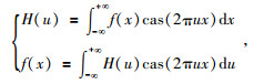
|
(1) |
其中cas(2πux)=cos(2πux)+sin(2πux).
对于二维Hartley变换的定义,存在两种不同的形式,其区别在于积分核不同.Sundararajan(1995)曾对此进行讨论,根据Bracewell(2000)的建议,本文采用标准形式的二维Hartley变换,则二维连续实函数f(x, y)的Hartley变换及其逆变换定义为
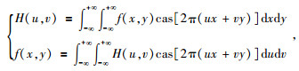
|
(2) |
其中cas[2π(ux+vy)]=cos[2π(ux+vy)]+sin2π(ux+vy)].
可以看出,Hartley变换及其逆变换具有完全相同的形式,构成了严格对称的变换,并且Hartley变换在实数域空间进行.
而对于一维函数f(x)的Fourier变换及其逆变换定义为(布隆什坦和谢缅佳也夫,1965)
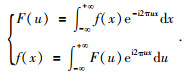
|
(3) |
对于二维函数f(x, y)的Fourier变换及其逆变换定义为
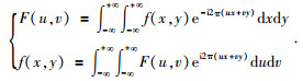
|
(4) |
从Fourier变换和Hartley变换的定义形式对比可以看出,二者定义形式基本相似.Hartley正、反变换定义式具有完全相同的核函数,且为实数;而Fourier正、反变换定义式中的核函数互为共轭,且为复数.
(2) Hartley变换和Fourier变换的性质
Hartley变换具有与Fourier变换相似的特征,也拥有Fourier变换相似的大部分性质(甘利灯,1992).下面给出一维和二维Hartley变换的性质.
设一维连续实函数f(x)、f1(x)和f2(x),其Hartley变换为H(u)=HT[f(x)],H1(u)=HT[f1(x)],H2(u)=HT[f2(x)],其Fourier变换为F(u)=FT[f(x)],F1(u)=FT[f1(x)],F2(u)=FT[f2(x)].其中u是x方向的频率,“HT”代表Hartley变换算子,“FT”代表Fourier变换算子,表 1给出了一维Hartley变换和Fourier变换的性质(甘利灯,1992).
|
|
表 1 一维Hartley变换与Fourier变换性质对比表 Table 1 The contrast table of properties of 1D Hartley transform and Fourier transform |
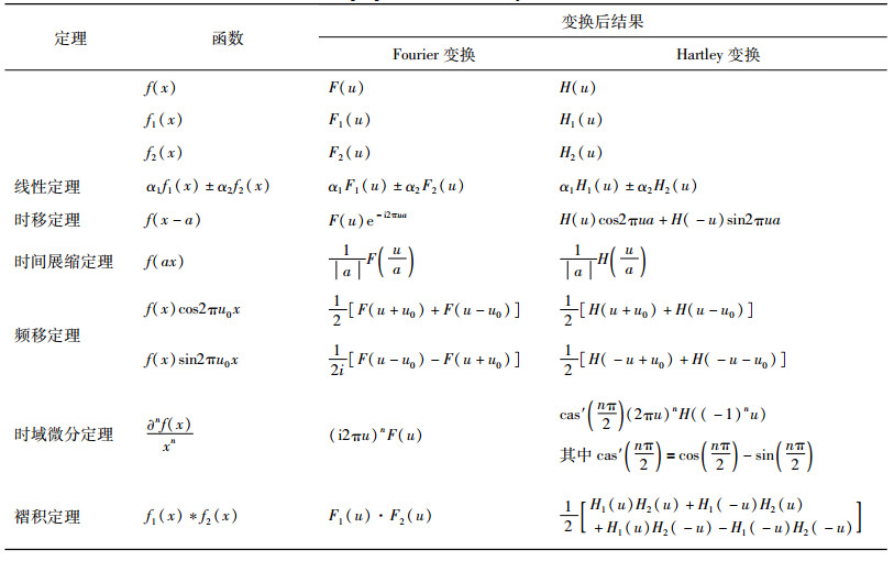
设二维连续实函数f(x, y)、f1(x, y)和f2(x, y),其Hartley变换谱分别为H(u, v)=HT[f(x, y)],H1(u, v)=HT[f1(x, y)],H2(u, v)=HT[f2(x, y)],其Fourier变换谱分别为F(u, v)=FT[f(x, y)],F1(u, v)=FT[f1(x, y)],F2(u, v)=FT[f2(x, y)],其中,u、v分别是x和y方向的频率.“HT”作为Hartley变换算子,“FT”作为Fourier变换算子,表 2给出了二维Hartley变换与Fourier变换的性质(甘利灯,1992).
|
|
表 2 二维Hartley变换与Fourier变换性质对比表 Table 2 The contrast table of properties of 2D Hartley transform and Fourier transform |

从表 1和表 2可以看出,Hartley变换的时移定理、频移定理、时域微分定理和褶积定理均需将原来的频谱做关于零频的对称谱,然后对其频谱和对称谱均乘以相应的因子才可得到相应变换后的结果;而基于Fourier变换的性质不需要求取关于零频的对称谱.但对于褶积定理而言,当实函数f1(x, y)和f2(x, y)中有一个函数为偶函数时,那么这两个函数的Hartley变换褶积频谱与Fourier变换褶积频谱形式相同(Saatcilar et al., 1990),即HT[f1(x, y)×f2(x, y)]=H1(u, v)·H2(u, v).因此,通过Fourier变换和Hartley变换性质对比可以发现,Fourier变换的大部分性质比Hartley变换的性质更加简洁.
(3) Hartley变换和Fourier变换快速算法的计算量
设Me表示实乘运算次数,Ae表示实加运算次数,M=2s和N=2t为点数.则一维快速Fourier变换的计算量分别为(蒋增荣等,1993)
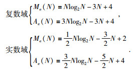
|
二维快速Fourier变换的计算量分别为(蒋增荣等,1993)
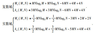
|
一维、二维快速Hartley变换的计算量分别为(成礼智,1988)
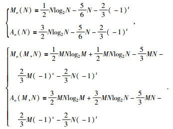
|
通过快速Hartley变换计算量与快速Fourier变换计算量对比可得,实数域快速Fourier变换计算量约为复数域快速Fourier变换计算量的一半,近似与快速Hartley变换计算量相当.
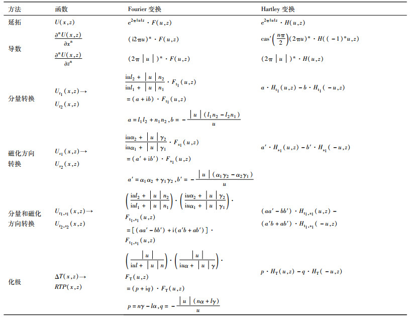
2 基于Hartley变换和Fourier变换的位场数据处理和转换频率响应对比这里的位场转换包括位场延拓、各阶方向导数转换、重磁异常分量转换和磁异常磁化方向转换.
设Ut1(x, y, z),Ut2(x, y, z)分别为位函数U(x, y, z)在单位矢量t1=(l1, m1, n1)和t2=(l2, m2, n2)方向的位场分量.Us1(x, y, z),Us2(x, y, z)分别表示同一分量在单位矢量s1=(α1, β1, γ1)和s2=(α2, β2, γ2)磁化方向的磁异常.Ut, s(x, y, z)表示地磁场方向为t =(l, m, n)和磁化方向为s =(α, β, γ)的磁异常分量.则有关Fourier变换和Hartley变换在位场数据处理和转换中的频率响应对比见表 3和表 4(据侯重初和刘秀芳,1978;魏雅利和骆遥,2010;骆遥,2013)所示.
|
|
表 3 一维Hartley变换和Fourier变换在位场数据处理和转换中的频率响应对比表 Table 3 The contrast table of frequency response based on 1D Hartley transform and Fourier transform in potential field data processing and transformation |
|
|
表 4 二维Hartley变换和Fourier变换在位场处理和转换中的频率响应对比表 Table 4 The contrast table of frequency response based on 2D Hartley transform and Fourier transform in potential field data processing and transformation |
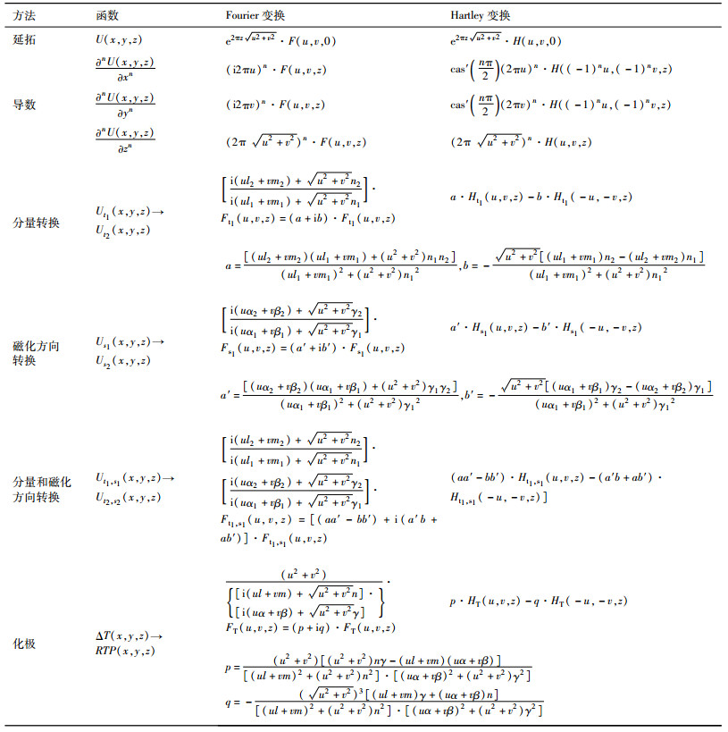
综上,Hartley变换和Fourier变换的位场延拓表达式相同,Hartley变换的导数因子和方向转换因子要比Fourier变换的复杂.总的来说,在位场数据处理和转换中,Fourier变换的频谱响应表达式要比Hartley变换的频谱响应表达式更加简洁.
3 理论模型测试为了验证Hartley变换在位场数据处理和转换中的计算精度和计算时间,我们设计了单一直立六面体模型(图 1)进行测试,模型长、宽范围分别为-400~400 m(图中白色边框为模型的具体位置),顶深50 m,厚750 m,模型体密度为0.7×10³ kg/m3,磁化强度为1.0 A/m,地磁场偏角为5°,倾角为50°.计算面为z=0平面规则网,计算点的变化范围在x方向上从-1000~1000 m,点距为10 m;y方向从-1000~1000 m,点距为10 m.图 1给出了在z=0 m处的理论重力异常平面图,图 2给出了在z=0 m处的理论磁力异常平面图,所有模型测试的扩边方法均用最小曲率扩边方法(王万银等,2009).

|
图 1 理论模型重力异常平面图 Figure 1 The plane map of the theoretical model's gravity anomaly |

|
图 2 理论模型ΔT磁异常平面图 Figure 2 The plane map of the theoretical model's ΔT magnetic anomaly |
(1) 位场解析延拓测试
为了验证Fourier变换和Hartley变换在位场解析延拓中的计算精度和计算时间.我们选取了观测面为z=0 m处的理论重力异常,分别向上延拓20 m和向下延拓20 m的重力异常,计算结果如图 3所示.

|
图 3 Fourier变换和Hartley变换重力异常延拓平面图 (a)和(d)分别为高度-20 m和20 m的理论重力异常;(b)和(c)分别为基于Hartley变换和Fourier变换的重力异常向上延拓20 m的结果;(e)和(f)分别为基于Hartley变换和Fourier变换的重力异常向下延拓20 m的结果. Figure 3 The plane map of the continued gravity anomaly based on Fourier transform and Hartley transform (a) and (d)Are the theoretical gravity anomaly in -20 m and 20 m; (b) and (c) Are the continued gravity anomaly based on Fourier transform and Hartley transform in -20 m, respectively; (e) and (f) Are the continued gravity anomaly based on Fourier transform and Hartley transform in 20 m, respectively. |
图 3a是向上延拓20 m的理论重力异常平面图,图 3b和图 3c分别是对图 1所示重力异常利用Fourier变换和Hartley变换向上延拓20 m的重力异常平面图.图 3d是向下延拓20 m的理论重力异常图,图 3e和图 3f分别是对图 1所示重力异常利用Fourier变换和Hartley变换向下延拓20 m的重力异常平面图.从图 3对比发现,Fourier变换与Hartley变换的延拓结果基本相同.通过计算Fourier变换和Hartley变换向上延拓20 m的重力异常与该高度的理论重力异常的均方误差分别0.066×10⁻⁶ m/s2和0.065×10-6 m/s2,Fourier变换与Hartley变换向下延拓20 m的重力异常与该高度的理论重力异常的均方误差分别为0.152×10⁻⁶ m/s2和0.151×10-6 m/s2.从均方误差上可以看出其计算精度相近.就计算量而言,实数域Fourier变换与Hartley变换的计算时间大约分别为0.802 s和0.796 s(计算机配置:内存4 GB,处理器Intel(R)Core(TM)i5 CPU 760 @ 2.80 GHz 2.79 GHz,显卡ATI Radeon HD 5750,下同).因此,Hartley变换与实数域Fourier变换位场延拓具有相同的精度,且计算时间也基本相同.
(2) 位场导数转换测试
为了对比Fourier变换和Hartley变换位场导数计算精度和计算时间,我们选用图 1理论重力异常,分别利用Hartley变换和Fourier变换计算x、y和z方向一阶导数(图 4).从图 4可以看出,Hartley变换与Fourier变换位场导数计算结果基本相同.Fourier变换在计算x、y和z方向一阶导数结果与理论异常导数之间的均方误差分别为1.51×10⁻⁴ s-2,1.51×10-4 s-2,3.39×10-3 s-2,Hartley变换在计算x、y和z方向一阶导数结果与理论异常导数之间的均方误差分别为1.51×10⁻⁴ s-2,1.50×10-4 s-2,3.39×10-3 s-2.实数域Fourier变换和Hartley变换位场导数转换所用时间(x,y,z方向导数计算时间基本相同)分别为0.792 s和0.780 s.因此,Hartley变换与Fourier变换在位场导数计算方面具有相同的计算精度,且与实数域Fourier变换计算时间基本相同.

|
图 4 Fourier变换和Hartley变换重力异常导数转换结果平面图 (a),(b)和(c)分别是水平x方向一阶导数理论值,Fourier变换和Hartley变换计算结果;(d),(e)和(f)分别是水平y方向一阶导数理论值,Fourier变换和Hartley变换计算结果;(g),(h)和(i)分别是z方向一阶导数理论值,Fourier变换和Hartley变换计算结果. Figure 4 The plane map of the derivative transformation of gravity anomaly based on Fourier transform and Hartley transform (a), (b) and (c) Are theoretical, Fourier transform and Hartley transform of gravity anomalies about horizontal x direction first order derivative, respectively; (d), (e) and (f) Are theoretical, Fourier transform and Hartley transform of gravity anomalies about horizontal y direction first order derivative, respectively; (g), (h) and (i) Are theoretical, Fourier transform and Hartley transform of gravity anomalies about vertical z direction first order derivative, respectively. |
(3) 磁异常分量转换和磁化方向转换测试
根据图 2所示磁力异常进行化极处理,理论化极磁异常如图 5a所示.图 5b和图 5c分别是基于Fourier变换和Hartley变换得到的化极磁异常,从图 5可以看出,Fourier变换和Hartley变换的化极磁异常基本相同.我们也计算了频率域化极磁异常与理论化极磁异常之间的均方差,实数域Fourier变换化极与理论化极磁异常之间的均方差为4.395 nT,Hartley变换化极与理论化极磁异常之间的均方差为4.394nT,从均方差可以看出,Hartley变换化极与Fourier变换化极具有相同的精度.在计算时间上,实数域Fourier变换用时0.802 s,Hartley变换化极用时0.794 s,可以看出Hartley变换与实数域Fourier变换计算时间基本相同.

|
图 5 Fourier变换和Hartley变换磁异常化极结果平面图 (a),(b)和(c)分别是理论,Fourier变换和Hartley变换化极磁异常. Figure 5 The plane map of the reduction-to-the-pole magnetic anomaly based on Fourier transform and Hartley transform (a), (b) and (c) Are the Theoretical, Fourier transform and Hartley transform reduction-to-the-pole magnetic anomaly, respectively. |
本次实际资料处理选取我国某地调平后的航磁资料进行处理,现给出实际资料的总场磁异常如图 6所示,然后利用Hartley变换和Fourier变换方法对该区的实际资料进行处理,从而比较Hartley变换和Fourier变换在位场处理和转换方面的效果,实际资料处理扩边方法均用最小曲率扩边方法.(王万银等,2009)

|
图 6 ΔT磁力异常平面图 Figure 6 The plane map of ΔT magnetic anomaly |
(1) 位场解析延拓
利用Fourier变换和Hartley变换对图 6所示磁异常进行解析延拓.图 7a、图 7b是利用Fourier变换向上延拓300 m和向下延拓300 m的磁异常结果,图 7c和图 7d是利用Hartley变换向上延拓300 m和向下延拓300 m的磁异常结果.从图中可以发现,Hartley变换与Fourier变换位场延拓结果基本相同,在向上延拓中,Fourier变换与Hartley变换之间偏差的均方差为0.0956 nT,在向下延拓中,Fourier变换与Hartley变换之间偏差的均方差为0.158nT,这个偏差是由于数值计算误差造成,而不是方法本身造成.

|
图 7 Fourier变换和Hartley变换磁异常延拓平面图 (a)和(c)分别是基于Fourier变换和Hartley变换的磁异常向上延拓300 m结果;(b)和(d)分别是基于Fourier变换和Hartley变换的磁异常向下延拓300 m结果. Figure 7 The plane map of continuation magnetic anomaly based on Fourier transform and Hartley transform (a) and (c) Are continued magnetic anomaly based on Fourier transform and Hartley transform in -300 m, respectively; (b) and (d) Are continued magnetic anomaly based on Hartley transform and Hartley transform in 300 m, respectively. |
在计算时间上,实数域Fourier变换所用时间为0.754 s,Hartley变换所用时间0.733 s.可以看出Hartley变换所用时间与实数域Fourier变换基本相同,其精度也相同.
(2) 位场导数计算
分别利用Fourier变换和Hartley变换计算图 6所示磁异常x、y、z方向一阶导数(图 8).从计算结果可以看出,Fourier变换和Hartley变换各方向导数计算结果基本相同.Hartley变换和Fourier变换位场导数在x、y和z三个方向一阶导数之间偏差的均方差分别为7.23×10⁻⁶ nT/m、5.61×10-6 nT/m和1.45×10-4 nT/m.就计算量而言,Hartley变换和实数域Fourier变换的计算时间分别为0.7488 s和0.7686 s.因此,从计算结果可以看出,Hartley变换位场导数与Fourier变换位场导数处理结果基本相同,两者之间的偏差均方误差较小,表明这两种方法得到的计算结果基本相同;从计算时间来看,Hartley变换与实数域Fourier变换计算时间基本相同.

|
图 8 Fourier变换和Hartley变换磁异常导数转换结果平面图 (a),(c)和(e)分别是基于Fourier变换的x、y和z方向的一阶导数计算结果;(b),(d)和(f)分别是基于Hartley变换的x、y和z方向的一阶导数计算结果. Figure 8 The plane map of the derivative transformation of magnetic anomaly based on Fourier transform and Hartley transform (a), (c) and (e) Are the derivative of magnetic anomaly based on Fourier transform about x, y and z, respectively; (b), (d) and (f) Are the derivative of magnetic anomaly based on Hartley transform about x, y and z, respectively. |
(3) 磁异常化极处理
对于磁异常分量转换和磁化方向转换,利用Fourier变换和Hartley变换对图 6所示磁力异常进行化极处理(图 9).通过对比发现,Fourier变换与Hartley变换化极结果基本相同,Hartley变换与Fourier变换之间的偏差均方差为0.0401 nT.在计算时间上,实数域Fourier变换用时0.8654 s,Hartley变换用时0.8634 s.因此,Fourier变换与Hartley变换所需计算时间基本相同,其精度也基本相同.

|
图 9 Fourier变换和Hartley变换化极磁异常平面图 (a)和(b)分别为Fourier变换和Hartley变换化极磁异常结果. Figure 9 The plane map of reduction-to-the-pole magnetic anomaly based on Fourier transform and Hartley transform (a) and (b) Are reduction-to-the-pole magnetic anomaly base on Fourier transform and Hartley transform respectively. |
通过整理Hartley变换与Fourier的定义、性质、快速算法的计算量以及在位场数据处理和转换上的频率域响应,对Hartley变换和Fourier变换进行对比研究.通过对比认为,Hartley变换的性质、频率响应比Fourier变换复杂,Hartley变换的快速算法与实数域Fourier变换的快速算法计算量基本相同;通过理论模型测试得出其计算精度基本相同;通过理论模型测试和实际资料处理试验验证了其计算量基本相同.
5.2因此,在位场数据处理和转换中,由于Hartley变换比Fourier变换的频率响应复杂,而且其快速算法的计算量和计算精度基本相当,从使用的角度来看,Fourier变换更具有优势.
致谢 感谢论文评审专家和潘作枢教授提出的修改意见,也感谢本文编辑对论文的加工和修改.| [] | Al-Garni Mansour A, Sundararajan N. 2012. Hartley spectral analysis of self-potential anomalies caused by a 2-D horizontal circular cylinder[J]. Arabian Journal of Geosciences, 5(6): 1341–1346. DOI:10.1007/s12517-011-0285-8 |
| [] | Bracewell R N. 1983. Discrete Hartley transform[J]. J. Opt. Soc. Am., 73(12): 1832–1835. DOI:10.1364/JOSA.73.001832 |
| [] | Bracewell R N. 1984. The fast Hartley transform[J]. Proc. IEEE, 72(8): 1010–1018. DOI:10.1109/PROC.1984.12968 |
| [] | Bracewell R N. 1986. The Hartley Transform[M]. New York: Oxford University Press. |
| [] | Bracewell R N. 2000. The Fourier Transform and its Applications[M]. 3rd ed. New York: McGraw-Hill. |
| [] | Cheng L Z. 1988. A fast discrete Hartley Transform algorithm[J]. Numerical computation and computer application(3): 162–168. |
| [] | Gan L D. 1992. Hartley transform and its properties[J]. Oil Geophysical Prospecting (in Chinese), 27(5): 605–616. |
| [] | Hartley R V L. 1942. A more symmetrical Fourier analysis applied to transmission problems[J]. Proc. IRE, 30(3): 144–150. DOI:10.1109/JRPROC.1942.234333 |
| [] | Hou H S. 1987. The fast Hartley transform algorithm[J]. IEEE Trans. Comp., C-36(2): 147–156. DOI:10.1109/TC.1987.1676877 |
| [] | Hou Z C, Liu X F. 1978. Potential field transform of gravity and magnetic data by Fourier transform[J]. Journal of Beijing Normal University (Natural Science)(2): 54–69. |
| [] | Jiang Z R, Zeng Y H, Yu P N. 1993, Fast algorithm(in Chinese)[M], Chang sha:National University of Defence Technology Press, 87-100. |
| [] | Kadirov F A. 2000. Application of the Hartley transform for interpretation of gravity anomalies in the Shamakhy-Gobustan and Absheron oil-and gas-bearing regions, Azerbaijan[J]. J. Appl. Geophys., 45(1): 49–61. DOI:10.1016/S0926-9851(00)00018-5 |
| [] | LiYaoguo, Oldenburg D W. 1998. Fast inversion of large scale magnetic data using wavelet[J]. Yuan G Q Trans. Journal of Beijing Normal University (in Chinese)(4): 23–28. |
| [] | LiZ J, Yang L, Wang Q C. 1997. Application of the wavelet transform in potential field data processing[J]. Geophysical Prospecting for Petroleum (in Chinese), 36(2): 86–93. |
| [] | Liu Y X, Zhang L B, Zhao Z F, et al. 1993. Interborehole acoustic wave field simulation using the Hartley transform[J]. Oil Geophysical Prospecting (in Chinese), 28(3): 276–281. |
| [] | Luo Y, Wang M, Luo F, et al. 2011. Direct analytic signal interpretation of potential field data using 2-D Hilbert transform[J]. Chinese J. Geophys. (in Chinese), 54(7): 1912–1920. DOI:10.3969/j.issn.0001-5733.2011.07.025 |
| [] | Luo Y. 2013. Hartley transform for reduction to the pole[J]. Chinese J. Geophys. (in Chinese), 56(9): 3163–3172. DOI:10.6038/cjg20130929 |
| [] | Ma G Q, Huang D N, Du X J, et al. 2014. Hartley transform in the application of the derivatives of potential field (gravity and magnetic) data[J]. Journal of Jilin University (Earth Science Edition) (in Chinese), 44(1): 328–335. |
| [] | Marobhe I M. 1990. Application of the Hartley transform to the interpretation of magnetic anomalies due to two-dimensional dyke bodies[J]. Geoexploration, 26(4): 291–301. DOI:10.1016/0016-7142(90)90009-H |
| [] | Miao L C. 1993. Application of Hartley transform to numerical modeling[J]. Oil Geophysical Prospecting (in Chinese), 28(1): 91–96. |
| [] | Mohan N L, Sundararajan N, Seshagiri Rao S V. 1982. Interpretation of some two-dimensional magnetic bodies using Hilbert transforms[J]. Geophysics, 47(3): 376–387. DOI:10.1190/1.1441342 |
| [] | Mu S M, Shen N H, Sun Y S. 1990. Application of method of regional geophysical data processing[M]. Changchun: Jilin Science and Technology Publishing. |
| [] | Nabighian M N. 1972. The analytic signal of two-dimensional magnetic bodies with polygonal cross-section: Its properties and use for automated anomaly interpretation[J]. Geophysics, 37(3): 507–512. DOI:10.1190/1.1440276 |
| [] | Nagendra R. 1984. The principle of complex frequency scaling-Applicability in inclined continuation of potential fields[J]. Geophysics, 15(4): 2019–2023. |
| [] | Rao B N, Krishna P R, Markandeyulu A. 1996. MAPROS-a computer program for basement mapping and filtering of gravity and magnetic data using a Hartley transform[J]. Computers & Geosciences, 22(3): 197–218. |
| [] | Saatcilar R, Ergintav S, Canitez N. 1990. The use of the Hartley transform in geophysical applications[J]. Geophysics, 55(11): 1488–1495. DOI:10.1190/1.1442796 |
| [] | Saatcilar R, Ergintav S. 1991. Solving elastic wave equations with the Hartley method[J]. Geophysics, 56(2): 274–278. DOI:10.1190/1.1443040 |
| [] | Stanley J M, Green R. 1976. Gravity gradients and the interpretation of the truncated plate[J]. Geophysics, 41(6): 1370–1376. DOI:10.1190/1.1440687 |
| [] | Sundararajan N. 1995. 2-D Hartley transforms[J]. Geophysics, 60(1): 262–267. DOI:10.1190/1.1443754 |
| [] | Sundararajan N, Brahmam G R. 1998. Spectral analysis of gravity anomalies caused by slab-like structures: A Hartley transform technique[J]. J. Appl. Geophys., 39(1): 53–61. DOI:10.1016/S0926-9851(97)00041-4 |
| [] | Wang W Y, Qiu Z Y, Liu J L, et al. 2009. The research to the extending edge and interpolation based on the minimun curvature method in potential field data processing[J]. Progress in Geophys. (in Chinese), 24(4): 1327–1338. DOI:10.3969/j.issn.1004-2903.2009.04.022 |
| [] | Wei Y L, Luo Y. 2010. 2D potential field transformation based on Hartley transform[J]. Progress in Geophys (in Chinese), 25(6): 2102–2108. DOI:10.3969/j.issn.1004-2903.2010.06.029 |
| [] | Wu X Z, Liu G H, Xue G Q, et al. 1987. Application of Fourier transform and field spectrum analysis method[M]. Beijing: Surveying and Mapping Publishing. |
| [] | Yao D Z, Ruan Y Z, Zhou X R. 1994. Elastic wave reverse time migration using Hartley transform[J]. Oil Geophysical Prospecting (in Chinese), 29(1): 19–22. |
| [] | Zhang F X, Meng L S, Zhang F Q, et al. 2005. Calculating normalized full gradient of gravity anomaly using Hilbert transform[J]. Chinese J. Geophys. (in Chinese), 48(3): 704–709. DOI:10.3321/j.issn:0001-5733.2005.03.031 |
| [] | Zhang F X, Meng L S, Zhang F Q, et al. 2006. A new method for spectral analysis of the potential field and conversion of derivative of gravity-anomalies: Cosine transform[J]. Chinese J. Geophys. (in Chinese), 49(1): 244–248. DOI:10.3321/j.issn:0001-5733.2006.01.031 |
| [] | Zhang F X, Zhang F Q, Meng L S, et al. 2007. Magnetic potential spectrum analysis and calculating method of magnetic anomaly derivatives based on discrete cosine transform[J]. Chinese J. Geophys. (in Chinese), 50(1): 297–304. DOI:10.3321/j.issn:0001-5733.2007.01.037 |
| [] | Zhang W S. 2003. Split-step Hartley transform prestack depth migration[J]. Geophysical Prospecting for Petroleum (in Chinese), 42(2): 149–153. |
| [] | Zhou H, He Q D. 1995. Seismic wave modeling in anisotropic medium by Hartley transform[J]. Oil Geophysical Prospecting (in Chinese), 30(5): 593–601, 614. |
| [] | Zhu W X, Tu W S, Liu T Y. 1989. Processing and interpretation of gravity and Magnetic Data[M]. Wuhan: China University of Geosciences Press. |
| [] | 布隆什坦, 谢缅佳也夫. 1965. 数学手册[M]. 罗零, 石峥嵘译. 北京: 高等教育出版社. |
| [] | 成礼智. 1988. 离散Hartley变换(DHT)及其快速算法[J].数值计算与计算机应用(3): 162–168. |
| [] | 甘利灯. 1992. 哈特莱变换及其性质[J].石油地球物理勘探, 27(5): 605–616. |
| [] | 侯重初, 刘秀芳. 1978. 用二维富氏变换进行重磁位场的转换[J].北京师范大学学报(自然科学版)(2): 54–69. |
| [] | 蒋增荣, 曾泳泓, 余品能. 1993. 快速算法[M]. 长沙: 国防科技大学出版社: 1-549. |
| [] | Li Y G, Oldenburg D W. 1998. 利用小波变换快速反演大型磁数据[J]. 袁桂琴译. 物探化探译丛, (4): 23-28. |
| [] | 李宗杰, 杨林, 王勤聪. 1997. 小波变换在位场数据处理中的应用[J].石油物探, 36(2): 86–93. |
| [] | 刘迎曦, 张霖斌, 赵振峰, 等. 1993. 利用哈特莱变换进行井间声波波场正演模拟[J].石油地球物探勘探, 28(3): 276–281. |
| [] | 骆遥, 王明, 罗锋, 等. 2011. 重磁场二维希尔伯特变换——直接解析信号解释方法[J].地球物理学报, 54(7): 1912–1920. DOI:10.3969/j.issn.0001-5733.2011.07.025 |
| [] | 骆遥. 2013. Hartley变换化极[J].地球物理学报, 56(9): 3163–3172. DOI:10.6038/cjg20130929 |
| [] | 马国庆, 黄大年, 杜晓娟, 等. 2014. Hartley变换在位场(重、磁)异常导数计算中的应用[J].吉林大学学报(地球科学版), 44(1): 328–335. |
| [] | 缪林昌. 1993. 哈特莱变换在数值模拟中的应用[J].石油地球物理勘探, 28(1): 91–96. |
| [] | 穆石敏, 申宁华, 孙运生. 1990. 区域地球物理数据处理方法及其应用[M]. 长春: 吉林科学技术出版社. |
| [] | 王万银, 邱之云, 刘金兰, 等. 2009. 位场数据处理中的最小曲率扩边和补差方法研究[J].地球物理学进展, 24(4): 1327–1338. |
| [] | 魏雅利, 骆遥. 2010. 基于Hartley变换的剖面位场转换[J].地球物理学进展, 25(6): 2102–2108. DOI:10.3969/j.issn.1004-2903.2010.06.029 |
| [] | 吴宣志, 刘光海, 薛光奇, 等. 1987. 富里叶变换和位场谱分析方法及其应用[M]. 北京: 测绘出版社. |
| [] | 尧德中, 阮颖铮, 周熙襄. 1994. Hartley变换法弹性波逆时偏移[J].石油地球物理勘探, 29(1): 19–22. |
| [] | 张凤旭, 孟令顺, 张凤琴, 等. 2005. 利用Hilbert变换计算重力归一化总梯度[J].地球物理学报, 48(3): 704–709. DOI:10.3321/j.issn:0001-5733.2005.03.031 |
| [] | 张凤旭, 孟令顺, 张凤琴, 等. 2006. 重力位谱分析及重力异常导数换算新方法—余弦变换[J].地球物理学报, 49(1): 244–248. DOI:10.3321/j.issn:0001-5733.2006.01.031 |
| [] | 张凤旭, 张凤琴, 孟令顺, 等. 2007. 基于离散余弦变换的磁位谱分析及磁异常导数计算方法[J].地球物理学报, 50(1): 297–304. DOI:10.3321/j.issn:0001-5733.2007.01.037 |
| [] | 张文生. 2003. 裂步Hartley变换叠前深度偏移[J].石油物探, 42(2): 149–153. |
| [] | 周辉, 何樵登. 1995. 利用Hartley变换模拟各向异性介质地震波场[J].石油地球物理勘探, 30(5): 593–601, 614. |
| [] | 朱文孝, 屠万生, 刘天佑. 1989. 重磁资料电算处理与解释方法[M]. 武汉: 中国地质大学出版社. |