重、磁方法是以地下介质物性差异(密度、磁性)为基础的一种地球物理勘探方法，本身具有成本低、周期短、效果好等特点，已成为查明地质构造、解决固体矿产资源和能源(石油、天然气和煤)勘探、地震及地质灾害预测、环境及工程监测等方面问题不可缺少的重要手段.位场数据处理和转换在快速Fourier变换提出之前主要在空间域进行，从1965年快速Fourier变换(FFT)问世以后，由于频率域位场数据处理和转换有计算公式简单、计算效率高的特点，位场数据处理和转换主要在频率域(波数域)中进行，并取得了很多成果(侯重初和刘秀芳，1978；Nagendra，1984；吴宣志等，1987；朱文孝等，1989；穆石敏，1990).随着信号分析理论的发展与完善，位场数据处理和转换的方法不再局限于Fourier频谱分析的理论，已经发展到小波变换(何继善等，1997；Li and Oldenburg, 1997；李宗杰等，1997)、Hilbert变换(Nabighian，1972；Stanley and Green, 1976；Stanley，1976；Mohan and Sundararajan, 1982；张凤旭等，2005；骆遥等，2011)、Hartley变换(Sundararajan and Brahmam, 1998；Kadirov，2000；魏雅利和骆遥，2010；Al-Garni and Sundararajan, 2012；骆遥，2013；马国庆等，2014)、余弦变换(张凤旭等, 2005a, 2006；刘东甲等，2012；刘繁明等，2013)等信号分析领域中.

离散余弦变换(DCT)是由Ahmed等(1974)提出的，经过几十年的应用与发展，DCT有三种经典的快速算法：B.G.LEE算法(Lee，1984)、AAN算法(Arai et al，1988)和LLM算法(Loeffler et al，1989).在地球物理数据处理中，DCT主要应用于地震数据和图像压缩.在位场数据处理中，2005年张凤旭和张凤琴等利用余弦变换研究密度界面重力异常的正、反演问题，认为余弦变换法反演的常密度单界面理论模型的深度误差小于Fourier变换法反演的界面深度.2006年张凤琴和刘财等利用余弦变换研究了规则形体重力异常频谱特征及反演方法.同年，张凤旭等提出了基于离散余弦变换的匹配滤波方法，提高了重磁异常划分的精确性和可靠性.2007年张凤旭和张凤琴等将DCT应用到位场数据导数转换中，认为其精度大于DFT(离散Fourier变换).2008年张凤旭和张凤琴等提出了基于DCT的Euler法确定断层断点位置的反演方法.2009年，张凤旭等将DCT应用到磁异常化极中，取得了较好的效果.2013年刘繁明等人为了获得高精度全张量磁梯度数据，提出了一种基于离散余弦变换的频率域快速计算方法.虽然有作者认为在位场数据处理和转换中，余弦变换比Fourier变换更具有优势.但刘东甲等人(2012)指出，DCT法的磁异常导数转换精度明显高于DFT法的结论是错误的.因此，对DCT和DFT在位场数据处理和转换方面的对比研究就具有一定意义.

本文通过整理余弦变换和Fourier变换的定义、性质、计算量以及在位场数据处理和转换中的频率响应，并通过理论模型测试和实际资料处理试验来研究余弦变换和Fourier变换在位场数据处理和转换中的优劣.

(1) 余弦变换和Fourier变换的定义

对于实连续函数f(t)，其余弦正变换与逆变换定义为(布隆什坦和谢缅佳也夫，1965)：

(1)

对于实连续函数f(x, y)，其余弦正变换与逆变换定义为(布隆什坦和谢缅佳也夫，1965)：

(2)

对于一维函数f(x)的Fourier变换及其逆变换定义为(布隆什坦和谢缅佳也夫，1965)：

(3)

对于二维函数f(x, y)的Fourier变换及其逆变换定义为(布隆什坦和谢缅佳也夫，1965)：

(4)

从Fourier变换和余弦换的定义形式对比可以看出，二者定义形式基本相似.余弦正、反变换定义式具有完全相同的核函数，且为实数；而Fourier正、反变换定义式中的核函数互为共轭，且为复数.

(2) 余弦变换和Fourier变换的性质

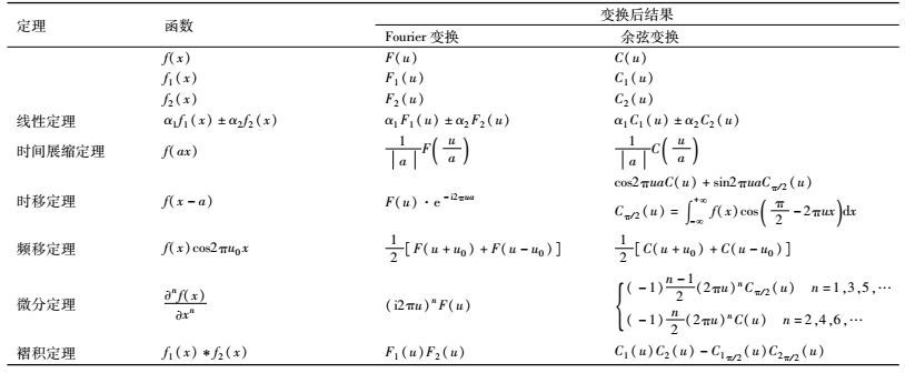
仿照Fourier变换的性质，余弦变换也有其相应的性质.表 1和表 2(布隆什坦和谢缅佳也夫，1965；张凤旭, 2006b, c, d)列出了一维和二维Fourier变换和余弦变换的性质.对比余弦变换和Fourier变换的性质，显然余弦变换的时间展缩性质和褶积性质受到函数奇偶性的影响，微分定理根据阶次的奇偶性具有不同的形式.整体来说，Fourier变换的大部分性质比余弦变换的性质更加简洁.

表 1 (Table 1)

表 1 一维余弦变换和Fourier变换基本性质对比表 Table 1 The contrast table of properties of 1D cosine transform and Fourier transform

表 1 一维余弦变换和Fourier变换基本性质对比表 Table 1 The contrast table of properties of 1D cosine transform and Fourier transform

表 2 (Table 2)

表 2 二维余弦变换和Fourier变换基本性质对比表 Table 2 The contrast table of properties of 2D cosine transform and Fourier transform

表 2 二维余弦变换和Fourier变换基本性质对比表 Table 2 The contrast table of properties of 2D cosine transform and Fourier transform

(3) 余弦变换和Fourier变换快速算法的计算量

设M_e表示实乘运算次数，A_e表示实加运算次数(蒋增荣等，1993)，则一维快速余弦变换算法的计算量为

(5)

二维快速余弦变换算法的计算量为

(6)

而一维快速Fourier变换算法的计算量为

二维快速Fourier变换算法的计算量为：

通过快速余弦变换与快速Fourier变换算法的计算量对比可得，实数域快速Fourier变换算法计算量基本是复数域计算量的一半，与快速余弦变换算法的计算量基本相当.

这里的位场转换包括位场延拓、各阶混合偏导数转换、重磁异常分量转换和磁异常磁化方向转换.设U_t1(x, y, z)和U_t2(x, y, z)分别为位函数U(x, y, z)在单位矢量t₁=(l₁, m₁, n₁)和t₂=(l₂, m₂, n₂)方向的位场分量.U_s1(x, y, z)和U_s2(x, y, z)分别表示同一分量在单位矢量s₁=(α₁, β₁, γ₁)和s₂=(α₂, β₂, γ₂)磁化方向的磁异常.U_{t, s}(x, y, z)表示分量方向为t=(l, m, n)和磁化方向为s=(α, β, γ)的磁异常.则有关Fourier变换和余弦变换在位场数据处理和转换中的频率响应对比见表 3和表 4(侯重初和刘秀芳，1978；张凤旭, 2006b, c, d，2007a, b, c)所示.

表 3 (Table 3)

表 3 一维余弦变换和Fourier变换在位场数据处理和转换中的频率响应对比表 Table 3 The contrast table of frequency response based on 1D cosine transform and Fourier transform in potential field data processing and transformation

表 3 一维余弦变换和Fourier变换在位场数据处理和转换中的频率响应对比表 Table 3 The contrast table of frequency response based on 1D cosine transform and Fourier transform in potential field data processing and transformation

表 4 (Table 4)

表 4 二维余弦变换和Fourier变换在位场数据处理和转换中的频率响应对比表 Table 4 The contrast table of frequency response based on 2D cosine transform and Fourier transform in potential field data processing and transformation

表 4 二维余弦变换和Fourier变换在位场数据处理和转换中的频率响应对比表 Table 4 The contrast table of frequency response based on 2D cosine transform and Fourier transform in potential field data processing and transformation

综上，余弦变换和Fourier变换的位场延拓因子相同，余弦变换的导数因子和方向转换因子要比Fourier变换的复杂.总的来说，在位场数据处理和转换中，Fourier变换的频谱响应公式要比余弦变换的频谱响应公式更加简洁.

本次试验选取一个直立六面体，其x方向坐标范围为-400~400 m，y方向坐标范围为-400~400 m，z方向(铅垂向下为正)坐标范围为50~850 m，剩余密度为0.7×10³ kg/m³，磁化强度为1.0 A/m，地磁场偏角为5°、倾角为50°.计算面为平面z=0(z坐标方向向下为正)，其在x方向上的坐标范围为-1000~1000 m，点距为10 m；在y方向上的坐标范围为-1000~1000 m，点距为10 m.图 1为z=0 m的重力异常平面图，图 2为z=0 m的磁力异常平面图，所有模型测试的扩边方法均采用最小曲率扩边方法(王万银等，2009).

图 1

Figure 1

图 1 模型重力异常平面图 Figure 1 The plane map of the theoretical model's gravity anomaly

图 2

Figure 2

图 2 模型ΔT磁异常平面图 Figure 2 The plane map of the theoretical model's ΔT magnetic anomaly

(1) 位场延拓测试

选取平面高度为0 m时的理论重力异常(图 1)为基准，分别把该平面上重力异常向上延拓20 m，向下延拓20 m，得到图 3所示重力异常，从重力异常图中可以看出FCT延拓结果和FFT延拓结果的重力异常图几乎一致.FCT和FFT向上延拓20m的重力异常与该高度的理论重力异常的均方误差分别为0.065×10^-6 m/s²和0.066×10^-6 m/s²，FCT和FFT向下延拓20 m的重力异常与该高度的理论重力异常的均方误差分别为0.150×10^-6 m/s²和0.152×10^-6 m/s².从均方误差上可以看出其计算精度相近.就计算量而言，FCT和实数域FFT的计算时间大约分别为0.33 s和0.34 s(计算机配置：内存64 GB，处理器intel(R)Xeon(R)CPU E5-2670 V3@ 2.30 GHz，显卡NVIDIA Quadro K620，下同)，因此FCT位场延拓所需计算量与实数域FFT的计算量基本相同.

图 3

Figure 3

图 3 FCT和FFT重力异常延拓平面图 (a)和(d)分别为高度-20 m和20 m的理论重力异常；(b)和(c)分别为基于FCT和FFT的重力异常向上延拓20 m的结果；(e)和(f)分别为基于FCT和FFT的重力异常向下延拓20 m的结果. Figure 3 The plane map of the continued gravity anomaly based on FCT and FFT (a) and (d) Are the theoretical gravity anomaly in -20 m and 20 m; (b) and (c) Are the continued gravity anomaly based on FCT and FFT in -20 m respectively; (e) and (f) Are the continued gravity anomaly based on FCT and FFT in 20 m respectively.

(2) 位场导数转换测试

根据图 1所示重力异常换算x，y，z三个方向的导数.图 4为基于FFT和FCT的重力异常导数转换结果.由该图可以看出，FCT和FFT的导数转换结果基本相同.FCT在x，y和z方向的导数转换结果与理论异常导数的均方误差分别为1.50×10^-4 s^-2，1.51×10^-4 s^-2和3.39×10^-3 s^-2，FFT在x，y和z方向的导数转换结果与理论异常导数的均方误差分别为1.51×10^-4 s^-2，1.51×10^-4 s^-2和3.39×10^-3 s^-2.FCT和实数域FFT的导数转换时间(x，y和z方向导数计算时间基本相同)分别为0.34 s和0.34 s.因此FCT在位场导数转换方面所需计算量与FFT的计算量基本相同，而且精度也基本相同.

图 4

Figure 4

图 4 FCT和FFT重力异常导数转换结果平面图 (a)，(b)和(c)分别为x，y和z方向理论导数；(d)，(e)和(f)分别为基于FCT的重力异常x，y和z方向导数转换结果；(g)，(h)和(i)分别为基于FFT的重力异常x，y和z方向导数转换结果. Figure 4 The plane map of the derivative transformation of gravity anomaly based on FCT and FFT (a), (b) and (c) Are the theoretical derivative of gravity anomaly about x, y and z respectively; (d), (e) and (f) Are the derivative of gravity anomaly based on FCT about x, y and z respectively; (g), (h) and (i) Are the derivative of gravity anomaly based on of FFT about x, y and z respectively.

(3) 磁异常分量转换和磁化方向转换测试

根据图 2所示磁力异常进行化极处理.图 5为基于FCT和FFT的磁异常化极结果.由图 5可以看出，基于FCT和FFT的磁异常化极结果相近，其均方误差分别为4.393 nT和4.395 nT.就计算量而言，FCT和实数域FFT的计算时间分别为0.34 s和0.35 s.因此FCT在位场分量转换和磁异常磁化方向转换方面所需计算量与FFT的基本相同，转换精度也基本相同.

图 5

Figure 5

图 5 FCT和FFT磁异常化极结果平面图 (a)为理论化极磁异常; (b)和(c)分别为基于FCT和FFT的化极磁异常. Figure 5 The plane map of the reduction-to-the-pole magnetic anomaly based on FCT and FFT (a)Is the theoretical reduction-to-the-pole magnetic anomaly; (b) and (c) Are the reduction-to-the-pole magnetic anomaly based on FCT and FFT respectively.

本次实际资料处理选取我国某地调平后的航磁资料(图 6)，然后利用FCT方法和FFT方法对该区的实际资料进行处理，从而比较FCT和FFT变换的效果及计算量，实际资料处理扩边方法均采用最小曲率扩边(王万银等，2009).

图 6

Figure 6

图 6 ΔT磁力异常平面图 Figure 6 The plane map of ΔT magnetic anomaly

(1) 磁异常解析延拓

分别利用FCT和FFT对上述实际磁异常分别向上延拓300 m和向下延拓300 m(图 7).由该图可以看出，基于FCT和FFT的位场延拓结果基本相同.向上延拓300 m时，FCT方法与FFT方法偏差的均方差为0.0957 nT；向下延拓300 m时，FCT方法与FFT方法偏差的均方差为0.157 nT，这个偏差是由于数值计算误差造成，而不是方法本身造成.就计算量而言，FCT和实数域FFT的计算时间分别为0.32 s和0.32 s.因此FCT和FFT在位场延拓所需的计算量基本相同，其精度也基本相同.

图 7

Figure 7

图 7 FCT和FFT磁异常延拓平面图 (a)和(b)分别为基于FCT和FFT的磁力异常向上延拓300 m的结果，(c)和(d)分别为基于FCT和FFT的磁力异常向下延拓300 m的结果. Figure 7 The plane map of the continued magnetic anomaly based on FCT and FFT (a) and (b) Are the continued magnetic anomaly based on FCT and FFT in -300 m respectively; (c) and (d) Are the continued magnetic anomaly based on FCT and FFT in 300 m respectively.

(2) 磁异常导数转换

分别利用FCT和FFT对图 6所示磁异常进行x、y和z方向的导数计算(图 8).由该图可以看出，基于FCT和FFT的位场导数转换结果基本一致，FCT和FFT在x、y和z三个方向偏差的均方差分别为7.27×10^-6 nT/m、5.99×10^-6 nT/m和1.44×10^-4 nT/m，与本身异常相比，这个偏差可以忽略.就计算量而言，FCT和实数域FFT的计算时间分别为0.34 s和0.34 s.因此FCT和实数域FFT在位场导数转换方面的计算精度基本相同，所需计算量也基本相同.

图 8

Figure 8

图 8 FCT和FFT磁异常导数转换结果平面图 (a)，(b)和(c)分别为基于FCT的x，y和z方向的导数；图(d)，(e)和(f)分别为基于FFT的x，y和z方向的导数. Figure 8 The plane map of the derivative transformation of magnetic anomaly based on FCT and FFT (a), (b) and (c) Are the derivative of magnetic anomaly based on FCT about x, y and z respectively; (d), (e) and (f) Are the derivative of magnetic anomaly based on FFT about x, y and z respectively.

(3) 磁异常化极处理

分别利用FCT和FFT对图 6所示磁异常进行化极处理(图 9).由该图可以看出，基于FCT和FFT的磁异常化极结果基本相同，FCT与FFT化极结果偏差的均方差为0.0396 nT.就计算量而言，FCT和实数域FFT的计算时间分别为0.34 s和0.34 s.因此，FCT和FFT所需计算时间基本相同，其精度也基本相同.

图 9

Figure 9

图 9 FCT和FFT磁异常化极结果平面图 (a)和(b)分别为FCT、FFT化极磁异常结果图. Figure 9 The plane map of the reduction-to-the-pole magnetic anomaly based on FCT and FFT (a) and (b) Are the reduction-to-the-pole magnetic anomaly based on FCT and FFT respectively.

综上，FCT和FFT两种方法在实际资料位场延拓、导数转换、分量和磁化方向转换方面的精度基本相同，所需计算量也基本相同.

通过整理余弦变换和Fourier变换的定义、性质、快速算法的计算量以及在位场数据处理和转换上的频率响应，对余弦变换和Fourier变换进行对比研究.通过对比认为，余弦变换的性质、频率响应比Fourier变换复杂，余弦变换的快速算法与实数域Fourier变换的快速算法计算量基本相同；通过理论模型测试得出其计算精度基本相同；通过理论模型测试和实际资料处理试验验证了其计算量基本相同.

因此，在位场数据处理和转换中，由于余弦变换比Fourier变换的频率响应复杂，而且其快速算法的计算量和计算精度基本相当，从使用的角度来看，Fourier变换更具有优势.