 2015, Vol. 30


2. 东华理工大学放射性地质与勘探技术国防重点学科实验室, 南昌 330013
2. Key Laboratory of Radioactive Geology and Exploration Technology Fundamental Science for National Defense, East China Institute of Technology, Nanchang 330013, China
电阻率法在环境、工程和水文等领域发挥了重要作用(Ramirez et al.,1996;Oldenburg et al.,1997;Kemna et al.,2002;汤洪志等,2003),取得了不错的成就,这与快速可靠的数据处理方法是分不开的.目前直流电一、二维反演计算已经很成熟,反演方法百花齐放(阮百尧等,1999;徐海浪和吴小平,2006;汤井田等,2008;韩波等,2012;程勃和底青云,2014),在实际应用中也取得了一定的应用效果,但是实际地质体通常是三维的,因此研究直流电三维正反演技术具有重要意义.近年来国内外学者对直流电阻率正反演作了深入的研究,提出了一系列反演方法,主要有基于Born近似的三维反演(Li and Oldenburg,1992,1994)、层析成像反演(Shima,1992)、Tarantola反演(Zhang et al.,1995)以及传统的最小二乘反演等方法(Sasaki,1994;Loke and Barker,1996;吴小平和徐果明,2000;黄俊革等,2007;刘斌等,2012).各种反演方法都有各自不同的模型约束,不同的模型约束反演的侧重点也不同.其中应用比较广泛的是基于最小构造或最平缓模型约束的反演(韩雪,2013;刘鑫明等,2013),这类反演方法能稳定收敛,但反演的地电图像是平滑的,有时不能分辨出地质界面,给后期的地质解释带来了一定的困难.基于全变差正则化反演(叶益信等,2009;韩波等,2012;叶益信等,2013)具有识别边界的能力,但反演结果对初始模型的依赖较大.
聚焦反演是一种对不同地质体界面进行反演成像方法,它的基本思想是将最小支撑泛函的稳定器与惩罚泛函相结合,引入一个新的稳定泛函来描述模型参数变化较大和不连续的区域,这样在反演中模型目标泛函会集中到最小的面积,从而显示出物性差别较大的界面.这一新方法已成功地应用到三维重力反演(Zhdanov,2002;Zhdanov et al.,2004;陈闫等,2014),三维磁力反演(Portniaguine and Zhdanov,2002)及大地电磁测深反演(Mehanee,2003;De Groot-Hedlin and Constable,2004;刘小军等,2007;Zhang et al.,2010)中,都取得了良好的应用效果.
本文将聚焦反演应用到直流电阻率三维反演中,通过对几个典型模型的试算,表明了该方法的有效性和可行性.
1 反演原理由于观测数据个数远小于模型参数的个数,地球物理反演问题通常是一个病态和不稳定问题,为了克服这个困难,通常采用Tikhonov正则化思想,即目标函数包括两部分,表示为
由于介质的电阻率变化范围很大,通常为了提高解的稳定性,反演中对模型参数取对数(ln(σ)),经这样变化后,变化范围很小,有利于反演的稳定.
在本文算法中,Wd采用如下形式的对角矩阵:
为了反映出物性差异较大的界面,提高反演结果的分辨率,本文引入最小支撑泛函作为模型的权函数,公式为
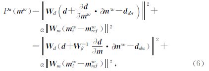
然后将最小化问题转化为加权模型空间形式,令 m w= W β m,m refw= W β m ref,在新的模型参数下,正演关系可表示为:


迭代后,未加权的模型参数为

该模型为一个大小为17 m×17 m×17 m、电阻率为200 Ω·m的均匀半空间含有一个大小为2.5 m×2.5 m×4 m、电阻率为10 Ω·m的低阻长方体模型,长方体顶部埋深为2 m,其z=4 m处的水平切片(XOY平面)如图 1a所示,y=0 m处的垂直切片(XOZ平面)如图 1b所示.模型剖分成40×40×20共32000个单元.

|
图 1 低阻模型4 m深度水平切片图(a)及y=0 m时垂直切片图(b) Fig. 1 A depth slice of the true model taken at 4-m depth(a) and a cross section of the true model taken at y=0(b)for low-resistivity model |
反演参考模型为200 Ω·m的均匀半空间,反演结果如图 2所示,图 2a和图 2b分别为光滑模型约束反演结果的水平切片和垂直切片,图 2c和图 2d分别为本文算法反演结果的水平切片和垂直切片,黑线框表示模型的边界位置.对比两种模式的反演结果可看出,光滑模型约束的反演结果在异常体位置出现了低阻异常值,低阻异常最小幅值在80 Ω·m左右,基本能够表征异常体的存在,但是异常范围偏大,成像聚焦效果较差,而本文算法反演结果低阻异常更明显,异常最小幅值在10 Ω·m左右,与真实异常体电阻率更接近,改善了低阻异常体的聚焦效果,对低阻异常体的定位更准确.

|
图 2 低阻模型光滑反演与聚焦反演结果比较
(a)光滑反演水平切片(z=4 m);(b)光滑反演垂直切片(y=0 m);(c)聚焦反演水平切片(z=4 m);(d)聚焦反演垂直切片(y=0 m). Fig. 2 Comparisons of focusing inversion with smoothing inversion for low-resistivity model (a)A depth slice of the smoothing inversion result taken at 4-m depth;(b)A cross section of the smoothing inversion result taken at y=0;(c)A depth slice of the focusing inversion result taken at 4-m depth;(b)A cross section of the focusing inversion result taken at y=0. |
图 3为两种反演方法的归一化迭代拟合差随迭代次数的变化情况,从中可看出,两种反演算法都能稳定收敛,但是聚焦反演的最终拟合差更小,迭代10次后聚焦反演归一化拟合差下降到10%左右,而光滑反演为20%左右,表明聚焦反演收敛速度更快.

|
图 3 低阻模型反演归一化拟合差曲线 Fig. 3 The normalized misfit curves with iteration inversions for low-resistivity model |
该模型为一个大小为17 m×17 m×17 m、电阻率为100 Ω·m的均匀半空间含有一个大小为2.5 m×2.5 m×4 m、电阻率为1000 Ω·m的高阻长方体模型,长方体顶部埋深为2 m,其z=4 m处的水平切片(XOY平面)如图 4a所示,y=0 m处的垂直切片(XOZ平面)如图 4b所示.模型剖分成40×40×20共32000个单元.

|
图 4 高阻体模型4 m深度水平切片图(a)及y=0 m时垂直切片图(b) Fig. 4 A depth slice of the true model taken at 4-m depth(a) and a cross section of the true model taken at y=0(b)for high-resistivity model |
反演参考模型为100 Ω·m的均匀半空间,反演结果如图 5所示,图 5a和图 5b分别为光滑模型约束反演结果的水平切片和垂直切片,图 5c和图 5d分别为本文算法反演结果的水平切片和垂直切片,黑线框表示模型的边界位置.对比两种模式的反演结果可看出,光滑模型约束的反演结果在异常体位置出现了高阻异常值,高阻异常最大值在150 Ω·m左右,基 本能够表征异常体的存在,但是整体聚焦效果较差,而本文算法反演结果高阻异常更明显,异常最大值在190 Ω·m 左右,与真实异常体电阻率更接近,高阻异常体的聚焦效果进一步提高,对高阻异常体的定位也更准确.相比低阻体模型,高阻体模型的反演电阻率与实际电阻率相差较大,而且对下底边界的拟合也相对较差,推测这是由于高阻对直流电法的屏蔽作用引起的.

|
图 5 高阻体模型光滑反演与聚焦反演结果比较
(a)光滑反演水平切片(z=4 m);(b)光滑反演垂直切片(y=0 m); (c)聚焦反演水平切片(z=4 m);(d)聚焦反演垂直切片(y=0 m). Fig. 5 Comparisons of focusing inversion with smoothing inversion for high-resistivity model (a)A depth slice of the smoothing inversion result taken at 4-m depth;(b)A cross section of the smoothing inversion result taken at y=0;(c)A depth slice of the focusing inversion result taken at 4-m depth;(b)A cross section of the focusing inversion result taken at y=0. |
图 6为两种反演方法的归一化迭代拟合差随迭代次数的变化情况,从中也可看出,两种反演算法都能稳定收敛,但是聚焦反演收敛速度更快,最终拟合差更小,进一步表明聚焦反演结果更接近真实模型.

|
图 6 高阻模型反演归一化拟合差曲线 Fig. 6 The normalized misfit curves with iteration inversions for the high-resistivity model |
本文将最小支撑泛函引入到电阻率法三维反演的目标函数中,然后采用高斯牛顿法求解反演目标函数最优化问题,同时结合预条件共轭梯度法得到电阻率法三维聚焦反演结果.
3.2通过两个模型的试算,本文算法反演结果增强了异常体成像的聚焦效果,也更好地框定了异常体的范围,该算法保留了光滑模型约束反演算法稳定、简单的特点,同时数据拟合程度得到进一步提高,表明本文反演算法具有稳定收敛、分辨率高、模型更聚焦等优点.但是该算法对模型的下底边界深度的反演拟合仍显不足,需要对模型的权矩阵或灵敏度矩阵作进一步改进研究.
致 谢 感谢审稿专家提出的宝贵修改意见和编辑部的大力支持!
| [1] | Chen Y, Li T L, Fan C S, et al. 2014. The 3D focusing inversion of full tensor gravity gradient data based on conjugate gradient[J]. Progress in Geophysics (in Chinese), 29(3): 1133-1142, doi: 10.6038/pg20140317. |
| [2] | Cheng B, Di Q Y. 2014. Statistic modeling 2D VES inversion in complex geo-electric structures[J]. Chinese J. Geophys. (in Chinese), 57(3): 961-967, doi: 10.6038/cjg20140325. |
| [3] | De Groot-Hedlin C, Constable S. 2004. Inversion of magnetotelluric data for 2D Structure with SHARP resistivity contrasts[J]. Geophysics, 69(1): 78-86. |
| [4] | Han B, Dou Y X, Ding L. 2012. Electrical resistivity tomography by using a hybrid regularization[J]. Chinese J. Geophys. (in Chinese), 55(3): 970-980, doi: 10.6038/j.issn.0001-5733.2012.03.027. |
| [5] | Han X. 2013. 3D DC resistivity inversion using weighted regularized conjugate gradient method (in Chinese) [D]. Changsha: Central South University. |
| [6] | Huang J G, Ruan B Y, Wang J L. 2007. The fast inversion for advanced detection using DC resistivity in tunnel[J]. Chinese J. Geophys. (in Chinese), 50(2): 619-624. |
| [7] | Kemna A, Kulessa B, Vereecken H. 2002. Imaging and characterisation of subsurface solute transport using electrical resistivity tomography (ERT) and equivalent transport models[J]. Journal of Hydrology, 267(3-4): 125-146. |
| [8] | Li Y G, Oldenburg D W. 1992. Approximate inverse mappings in DC resistivity problems[J]. Geophysical Journal International, 109(2): 343-362. |
| [9] | Li Y G, Oldenburg D W. 1994. Inversion of 3-D DC resistivity data using an approximate inverse mapping[J]. Geophysical Journal International, 116(3): 527-537. |
| [10] | Liu B, Li S C, Li S C, et al. 2012. 3D electrical resistivity inversion with least-squares method based on inequality constraint and its computation efficiency optimization[J]. Chinese J. Geophys. (in Chinese), 55(1): 260-268, doi: 10.6038/j.issn.0001-5733.2012.01.025. |
| [11] | Liu X J, Wang J L, Chen B, et al. 2007. Discussion on focus inversion algorithm of 2-D MT data[J]. Oil Geophysical Prospecting (in Chinese), 42(3): 338-342. |
| [12] | Liu X M, Liu S C, Jiang Z H, et al. 2013. Weighted smooth factor impact on 3D DC resistivity inversion and application in grouting effect detection[J]. Journal of China University of Mining & Technology (in Chinese), 42(1): 88-92. |
| [13] | Loke M H, Barker R D. 1996. Practical techniques for 3D resistivity surveys and data inversion[J]. Geophysical Prospecting, 44(3): 499-523. |
| [14] | Mehanee S A. 2003. Multidimensional finite difference electromagnetic modeling and inversion based on the balance method[D]. Utah: University of Utah. |
| [15] | Oldenburg D W, Li Y G, Ellis R G. 1997. Inversion of geophysical data over a copper gold porphyry deposit: a case history for Mt. Milligan[J]. Geophysics, 62(5): 1419-1431. |
| [16] | Portniaguine O, Zhdanov M S. 2002. 3-D magnetic inversion with data compression and image focusing[J]. Geophysics, 67(5): 1532-1541. |
| [17] | Ramirez A, Daily W, Binley A, et al. 1996. Detection of leaks in underground storage tanks using electrical resistance methods[J]. Journal of Environmental and Engineering Geophysics, 1(3): 189-203. |
| [18] | Ruan B Y, Yutaka M, Xu S Z. 1999. 2-D inversion programs of induced polarization data[J]. Computing Techniques for Geophysical and Geochemical Exploration (in Chinese), 21(2): 116-125. |
| [19] | Sasaki Y. 1994. 3-D resistivity inversion using the finite-element method[J]. Geophysics, 59(12): 1839-1848. |
| [20] | Shima H. 1992. 2-D and 3-D resistivity image reconstruction using crosshole data [J]. Geophysics, 57 (10): 1270-1281. |
| [21] | Tang H Z, Zhou Y D, Xu F, et al. 2003. Method and application examples of 2-D high- density resistivity imaging[J]. Journal of East China Geological Institute (in Chinese), 26(1): 87-90, 94. |
| [22] | Tang J T, Chen C, Quan C H, et al. 2008. A modified regularized inversion algorithm for electrical resistivity [J]. Computing Techniques for Geophysical and Geochemical Exploration (in Chinese), 30(4): 297-302. |
| [23] | Wu X P, Xu G M. 2000. Study on 3-D resistivity inversion using conjugate gradient method[J]. Chinese J. Geophys. (in Chinese), 43(3): 420-427, doi: 10.3321/j.issn:0001-5733.2000.03.016. |
| [24] | Xu H L, Wu X P. 2006. 2-D resistivity inversion using the neural network method[J]. Chinese J. Geophys. (in Chinese), 49(2): 584-589, doi: 10.3321/j.issn:0001-5733.2006.02.035. |
| [25] | Ye Y X, Hu X Y, Kim K, et al. 2009. Application analysis of sharp boundary inversion of magnetotelluric data for 2D structure[J]. Progress in Geophysics (in Chinese), 24(2): 668-674, doi: 10.3969/j.issn.1004-2903.2009.02.041. |
| [26] | Ye Y X, Deng J Z, Yang H Y, et al. 2013. SBI and RRI joint inversion of 2D magnetotelluric data and its applications[J]. Journal of East China Institute of Technology (in Chinese), 36(2): 204-209. |
| [27] | Zhang J, Mackie R L, Madden T R. 1995. 3-D dimensional resistivity forward modeling and inversion using conjugate gradients[J]. Geophysics, 60(5): 1313-1325. |
| [28] | Zhang L L, Yu P, Wang J L, et al. 2010. A study on 2D magnetotelluric sharp boundary inversion [J]. Chinese J. Geophys., 53(3): 631-637, doi: 10.3969/j.issn.0001-5733.2010.03.017. |
| [29] | Zhdanov M S. 2002. Geophysical Inverse Theory and Regularization Problems[M]. New York: Elsevier Science. |
| [30] | Zhdanov M S, Robert E, Souvik M. 2004. Three-dimensional regularized focusing inversion of gravity gradient tensor component data[J]. Geophysics, 69(4): 925-937. |
| [31] | 陈闫, 李桐林, 范翠松,等. 2014. 重力梯度全张量数据三维共轭梯度聚焦反演[J]. 地球物理学进展, 29(3): 1133-1142, doi: 10.6038/pg20140317. |
| [32] | 程勃, 底青云. 2014. 复杂地电结构条件下统计学建模法电阻率测深二维反演[J]. 地球物理学报, 57(3): 961-967, doi: 10.6038/cjg20140325. |
| [33] | 韩波, 窦以鑫, 丁亮. 2012. 电阻率成像的混合正则化反演算法[J]. 地球物理学报, 55(3): 970-980, doi: 10.6038/j.issn.0001-5733.2012.03.027. |
| [34] | 韩雪. 2013. 三维直流电阻率加权正则化共轭梯度反演[D]. 长沙: 中南大学. |
| [35] | 黄俊革, 阮百尧, 王家林. 2007. 坑道直流电阻率法超前探测的快速反演[J]. 地球物理学报, 50(2): 619-624. |
| [36] | 刘斌, 李术才, 李树忱,等. 2012. 基于不等式约束的最小二乘法三维电阻率反演及其算法优化[J]. 地球物理学报, 55(1): 260-268, doi: 10.6038/j.issn.0001-5733.2012.01.025. |
| [37] | 刘小军, 王家林, 陈冰,等. 2007. 二维大地电磁数据的聚焦反演算法探讨[J]. 石油地球物理勘探, 42(3): 338-342. |
| [38] | 刘鑫明, 刘树才, 姜志海,等. 2013. 电阻率三维反演中加权光滑因子的影响及注浆检测应用[J]. 中国矿业大学学报, 42(1): 88-92. |
| [39] | 阮百尧, 村上裕, 徐世浙. 1999. 电阻率/激发极化率数据的二维反演程序[J]. 物探化探计算技术, 21(2): 116-125. |
| [40] | 汤洪志, 周亚东, 徐飞,等. 2003. 高密度电阻率法二维成像方法及其应用[J]. 华东地质学院学报, 26(1): 87-90, 94. |
| [41] | 汤井田, 陈程, 全朝红,等. 2008. 一种改进的电阻率断面反演方法[J]. 物探化探计算技术, 30(4): 297-302. |
| [42] | 吴小平, 徐果明. 2000. 利用共轭梯度法的电阻率三维反演研究[J]. 地球物理学报, 43(3): 420-427, doi: 10.3321/j.issn:0001-5733.2000.03.016. |
| [43] | 徐海浪, 吴小平. 2006. 电阻率二维神经网络反演[J]. 地球物理学报, 49(2):584-589,doi:10.3321/j.issn:0001-5733.2006.02.035. |
| [44] | 叶益信, 胡祥云, 金钢燮,等. 2009. 大地电磁二维陡边界反演应用效果分析[J]. 地球物理学进展, 24(2): 668-674, doi: 10.3969/j.issn.1004-2903.2009.02.041. |
| [45] | 叶益信, 邓居智, 杨海燕,等. 2013. SBI与RRI结合的MT二维反演方法研究及应用[J]. 东华理工大学学报(自然科学版), 36(2): 204-209. |