居里温度是指磁性材料的自发磁化强度降低至零时的温度，在地球物理研究中，随深度增加，地球内部温度也增加，在达到一定温度时，地下物质出现退磁效应，这个温度称之为居里点，对应的深度称为居里面深度.岩石圈中的各类岩石因含有不同成分的铁磁性物质，在温度低于居里点时呈现出磁性，而磁性的强弱则与其含有的铁磁性物质的数量成正相关关系.在岩石圈，当温度到达居里点时，各类岩石磁性消失(铁磁性物质变为顺磁性而表现为无磁性)，此时由居里点组成的面即称为居里面.居里面之上，含铁磁性物质的岩石表现为有磁性，并产生磁异常场.研究居里面的分布，对认识地壳的深部构造、地热场的分布、油气成藏等具有重要意义.

基于居里面的基本性质，较直接的探测居里等温面的方法是根据大地热流值，地温与深度关系(Lachenbruch，1968；Negi，1987)来确定，但是这种方法在实际中并不常用. 最常用的方法是应用航磁和卫星磁数据.针对所研究的对象的不同，磁法又可以被分为两大类：独立磁异常法和整体磁异常法(Campos，1989；Enriquez，1990).这两大类下又可以有各种不同的应用技术，其中功率谱分析方法(Campos，1989；Enriquez，1990；Tanaka，1999；吴招才和高金耀，2010；高德章，2012)更为流行.整体磁异常的功率谱分析方法的理论基础是Spector&Grant统计模型，这个统计模型很适用于对区域磁异常整体的分析.

近年来，自相似和分形理论的应用为这一领域的研究提供了很多崭新的研究机会和科学思想.自相似法或分形模型可以认为是Spector&Grant方法(Spector和Grant，1970)的进一步发展.它考虑到了更加真实的磁异常分布.应用这一模型进行的学术研究都得到了不错的结果，并且揭示了之前研究方法中的局限性.

假设磁异常源，及磁性体的磁场分布具有白噪的功率谱(Hahn，1976)，磁化层在各个方向无限延伸，并且磁化强度M(x，y)是随机函数，利用Blakely(1995)和Tanaka等(1999)提出的方法，那么总磁场磁异常的功率谱(P)就可以表示为

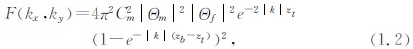
其中，P_M是磁化强度的功率谱，k_x和k_y是频率域的波数，k= k²_x+k²_y，z_t和z_b是磁异常源的上下边界.C_m为常数，Θ_m和Θ_f分别是磁场强度方向和地磁场方向的相关因子.

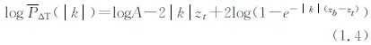
假设M(x，y)完全随机并不相关，则Φ_M(k_x，k_y)为常数，Θ_m和Θ_f的径向平均值为常数，深度因子e^{－2 k z_t}(1－e^{－ k(z_b－z_t)})²径向对称.因此P_ΔT的径向平均值可以简单的表示为

对方程(1.3)两边求对数，得

当波长小于两倍层厚度的时候，方程(1.4)可以近似为

这样，磁性层的上边界就可以通过上式估算得到.

假设z₀为磁性层的中间深度，则z₀=(z_t+z_b)/2，那么方程(1.3)可以表示为

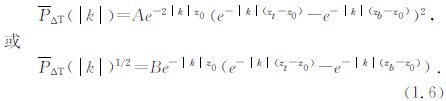
在长波长，即低波数波段范围内方程(1.6)可得到：

这里，B是常数，2d表示整个磁性层的厚度.

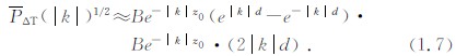
对P _ΔT(k)^1/2/ k 取对数，得

这样，通过方程(1.8)就可以得到磁性层的平均中心埋深.

那么，磁性层的底部深度，即居里面的深度就可以求出：

方程(1.5)和方程(1.8)成立的前提条件是磁异常源随机分布而且不相关，然而实际上磁异常源往往呈分形分布(Pilkington and Todoeschuck，1990，1994，2004;Maus and Dimr，1995，1996；Bansal et al.，1999，2001，2005，2010).考虑到这样的分布，很多人提出了新的求解方法，例如Pilkington and Todoeschuck(2004)；Pilkington等(1994)；Maus and Dimri(1996)； Dimri(2000)；Dimri等(2003)，等等.对于呈分形分布的磁异常源来讲，其磁场强度的径向平均功率谱满足：

其中β为分形指数，它的值取决于地下介质的岩性特征和不均匀性(Bansal等，2005).Pilkington and Todoeschuck(2004)；Pilkington等(1994)；Maus and Dimri(1996)；Maus等(1997)；Dimri(2000)均曾提出基于磁异常源分形分布的反演方法：通过比例常数，同时估算分形指数和功率谱，但是参数之间的相互关系却很难实现.于是Boulig and等(2009)提出了修正分形指数的方案，他们发现：火山地区的分形指数为2.0，在East Snake River平原大盆地的分形指数为2.5，科罗拉多高原为3.0，大峡谷为3.25(均为美国地区).

由于分形模型考虑到了更为真实的磁场强度差异的分形分布，因此自相似或分形模型是对Spector&Grant统计模型的完善和发展.

这里为了方便，记P _ΔT(k)为P(k)，结合方程(1.4)和方程(1.10)可以估算到中间深度为

上界面深度可通过方程(1.8)，(1.10)得到，即

假设磁异常源呈分形分布，变换方程(1.11)，(1.12)为如下形式：

然后同样是在低波数波段，通过基于最小二乘法的三维拟合求出z₀，z_t，β，进而利用方程(1.9)得到居里面深度.

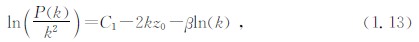
功率谱拟合的统计误差对结果准确性来说是一个重要参数，本文定义为：所选波段的实际数据与拟合所得数据之差的标准差除以角频率的范围(拟合时所选取的波段)(Tanaka，1999).公式为

其中σ[P(k)]为标准差：

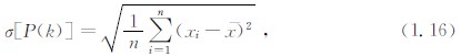
这里x_i为所选波段的实际数据与拟合所得数据之差，x 为x_i的平均值，n为所选波段数据的个数.

本文的实际数据来自于EMAG2(地球磁异常网格)(Maus，2009)，内容包括整个华北地区的地质构造，原始数据为二维磁异常数据.在图 1所示区域内磁场强度大，正负变化复杂，并且走向多变.从磁异常强度上看，中西部北纬40°附近的燕山造山带最强，且部分地区强弱变化大，局部磁异常发育呈正负相间的带状分布.在东部海域磁异常强度相对较小，正负变化较为平缓(周立宏等，2004).为了方便计算本文将原始数据进行横轴墨卡托投影变换，并重新将数据网格化处理，得到708×852大小的grd格式数据.

图 1

Fig. 1

图 1 华北地区磁异常图Fig. 1 The magnetic anomaly map in north of China

由于数据源比较大，利用surfer软件将整个数据分为西部(大小为294×482)、中部(大小为314×589)和东部(大小为261×551)三部分(图 1).

分别通过线性法和基于最小二乘法的三维拟合处理西中东三部分数据(假设层厚为20 km).

表 1(Table 1)

表 1 西部数据处理结果 Table 1 The result of the west data 方法 K1 K2 Zt估计值 Zt误差 K3 K4 Z0估计值 Z0误差 Zb估计值 方法1 0.1687 0.3552 12.2 km 0.6 km 0.0391 0.3048 20.7 km 0.8 km 29.2 km 方法2 0.1687 0.3263 10.9 km 0.8 km 0.0247 0.3119 11.0 km 0.4 km 11.0 km

表 1 西部数据处理结果 Table 1 The result of the west data

(1)线性法计算西部居里面深度

取西部数据做频谱计算，选取波段[0.1687，0.3552]拟合z_t，然后在波数域为[0.0391，0.3048]拟合z₀，得到如下结果(图 2)：

图 2

Fig. 2

图 2 线性法计算西部居里面深度Fig. 2 Calculate the depth of Curie point of west part by linear method

分别对能谱密度与角频率之比和角频谱在低波数域中进行直线拟合求斜率，得到顶部深度为12.2 km，误差0.6 km，平均深度为20.7 km，误差0.8 km，进而得到居里面深度为29.2 km.

(2)变换数据后进行三维拟合计算西部居里面深度

将β设为未知数，选取波段[0.1687，0.3263]拟合z_t，然后在波数域为[0.0247，0.3119]拟合z₀，得到以下结果(图 3):

图 3

Fig. 3

图 3 分形法计算西部居里面深度Fig. 3 Calculate the depth of Curie point of west part by scaling method

从matlab拟合结果中可以得到β等于2.78，磁异常层的顶部深度为10.9 km，误差0.8 km，平均深度为11.0 km，误差0.4 km，进而得到居里面深度为11.0 km.

表 2(Table 2)

表 2 中部数据处理结果 Table 2 The result of the middle data 方法 K1 K2 Zt估计值 Zt误差 K3 K4 Z0估计值 Z0误差 Zb估计值 方法1 0.1511 0.3660 12.9 km 0.4 km 0.0236 0.2920 21.6 km 0.9 km 30.2 km 方法2 0.1511 0.3660 8.7 km 0.3 km 0.0236 0.2920 12.4 km 0.4 km 16.1 km

表 2 中部数据处理结果 Table 2 The result of the middle data

(1)线性法计算中部居里面深度

取中部数据做频谱计算，选取波段[0.1511，0.3660]拟合z_t，然后在波数域为[0.0236，0.2920]拟合z₀，得到如下结果(图 4)：

图 4

Fig. 4

图 4 线性法计算中部居里面深度Fig. 4 Calculate the depth of Curie point of middle part by linear method

分别对能谱密度与角频率之比和角频谱在低波数域中进行直线拟合求斜率，得到顶部深度为12.9 km，误差0.4 km，平均深度为21.6 km，误差0.8 km，进而得到居里面深度为30.2 km.

(2)变换数据后进行三维拟合计算中部居里面深度

将β设为未知数，选取波段[0.1511，0.3660]拟合z_t，然后在波数域为[0.0236，0.2920]拟合z₀，得到以下结果(图 5):

图 5

Fig. 5

图 5 分形法计算中部居里面深度Fig. 5 Calculate the depth of Curie point of middle part by scaling method

从matlab拟合结果中可以得到β等于2.47，磁异常层的顶部深度为8.7 km，误差0.3 km，平均深度为12.4 km，误差0.4 km，进而得到居里面深度为16.1 km.

表 3(Table 3)

表 3 东部数据处理结果 Table 3 The result of the east data 方法 K1 K2 Zt估计值 Zt误差 K3 K4 Z0估计值 Z0误差 Zb估计值 方法1 0.1585 0.4426 10.4 km 0.5 km 0.0448 0.3452 18.5 km 0.7 km 26.7 km 方法2 0.1585 0.4426 8.8 km 0.4 km 0.0258 0.3208 9.4 km 0.4 km 10.0 km

表 3 东部数据处理结果 Table 3 The result of the east data

(1)线性法计算东部居里面深度

取东部数据做频谱计算，选取波段[0.1585，0.4426]拟合z_t，然后选取低波数波段[0.0448，0.3452]拟合z₀，然后求得z_b，得到如下结果(图 6)：

图 6

Fig. 6

图 6 线性法计算东部居里面深度Fig. 6 Calculate the depth of Curie point of east part by linear method

分别对能谱密度与角频率之比和角频谱在低波数域中进行直线拟合求斜率，得到顶部深度为10.4 km，误差0.5 km，平均深度为18.5 km，误差0.7 km，进而得到居里面深度为26.7 km.

(2)变换数据后进行三维拟合计算东部居里面深度

将β设为未知数，选取波段[0.1585，0.4426]拟合z_t，然后在波数域为[0.0258，0.3208]拟合z₀，得到以下结果(图 7):

图 7

Fig. 7

图 7 分形法计算东部居里面深度Fig. 7 Calculate the depth of Curie point of east part by scaling method

从matlab拟合结果中可以得到β等于3.02，磁异常层的顶部深度为8.8 km，误差0.4 km，平均深度为9.4 km，误差0.4 km，进而得到居里面深度为10.0 km.

通过将计算得到的结果与地热数据进行比较，分析何种方法更适用于该地区居里面深度的估算.下图为地下600摄氏度等深线图(图 8)：

图 8

Fig. 8

图 8 华北地区600摄氏度等深线图(据Wang，2006)Fig. 8 The contour map of 600-degree celsius in north China(From Wang，2006)

由图 2大概推测西部居里面深度在35 km左右，中部30 km左右，东部则是在25 km左右，与之前的方法相差不多(徐元芳等，1997).将其与由频谱分析方法得到的结果进行对比(表 4).

表 4(Table 4)

表 4 频谱分析处理结果与地热数据的对比 Table 4 Compare the results of Spectrum analysis and Geothermal data 西部 中部 东部 频谱分析 方法1 方法2 方法1 方法2 方法1 方法2 29.2 km 11.0 km 30.2 km 16.1 km 26.7 km 10.0 km 地热 35 km 30 km 25 km

表 4 频谱分析处理结果与地热数据的对比 Table 4 Compare the results of Spectrum analysis and Geothermal data

从地热角度来看，由西往东，地表热流值逐渐降低(臧绍先等，2002)，居里面深度呈递减趋势.对比由频谱分析法得到的结果，方法1，即线性拟合法更相符，而分形法则相差较多.可见利用磁异常估算居里面需要考虑不同方法的适用性，并与其他资料结合判断.华北地区地质演化复杂，东西中三部分有着不同的结构和演化史，地下结构横向差异变化较大，东部以渤海湾盆地为主，受到华北克拉通破坏影响严重，地层较薄，西部为鄂尔多斯盆地，其在华北克拉通是一完整的区块，较为稳定，中部造山带分隔了东西两个次级构造单元.受构造特征及演化历史影响，华北地区地热结构特征也存在较大差异，地下介质的组成及磁性特征受各类因素影响，对应磁异常场源分布规律也较为复杂.本文通过对不同模型条件下磁异常场源深度与地热特征的综合研究，表明该地区磁性场源与随机分布假设较为相近，华北地区平均居里面埋深约30 km，而且中西部较深，东部较浅.居里面反演结果也揭示了华北地区东西部结构差异较大，构造演化较为复杂，而东部渤海地区最浅，可能是由该地区地幔流动异常引起.

3.1    本文研究方法的理论基础是Spector和Grant(1970)统计模型，该模型是频谱分析法研究居里面深度的关键，无论是独立磁异常源的功率谱分析还是整个磁性体功率谱的分析都被广泛应用于居里面深度的计算当中.

3.2    若磁异常源呈随机分布且不相关时，可以利用线性法对磁性层顶部深度和平均深度进行拟合求解，进而得到磁性层底部深度即居里面深度；若磁异常源呈分形分布，则可以把分形系数作为未知数进行三维拟合的方法进行求解.分形模型是Spector & Grant方法的发展，它考虑到了真实的磁异常分布情况.

3.3    利用本文中的两种方法对华北地区磁异常数据进行处理，结合该地区的地热数据，分析、比较了两种方法的计算结果.结果表明：利用场源随机分布假设，线性法计算的居里面结果较为合理，与该地区地热数据较吻合.

致 谢 感谢审稿专家提出的修改意见和编辑部的大力支持！