 2015, Vol. 30


地球的岩石圈磁场属于地磁场的内源场之一,主要反映了岩石圈内部岩石磁性的三维空间分布.由于岩石的磁化环境(指岩石被磁化时的外部磁场及其随时间的变化)、温度-压力条件与磁性载体及其经历的地质作用与构造演化存在差异,岩石圈磁场携带着丰富的岩石矿物成分和岩石结构等地质构造信息,以及岩石所处温度与压力状态、深部岩石变质作用、构造运动与演化过程等地球动力学信息(e.g .Blakely,1995; Langel and Hinze,1998).因而,岩石圈磁场被广泛用于板块动力学及其演化历史重建、地震与火山等自然灾害的地质构造研究与预测和预报、金属矿产与油气藏资源勘探、地磁导航、大地构造与大陆动力学等领域( e.g. Mandea and Thébault,2007; ; 徐文耀等,2008a; Thébault et al.,2010; Purucker and Clark,2011).由此可知,岩石圈磁场的研究具有重要的地球科学理论意义、军事价值、经济价值与社会价值.
传统的地磁场观测平台和方式主要包括:地磁台连续观测、地磁台网多期重复观测、陆地表面移动式磁测、船载磁测、海底磁测、井中磁测、航空磁测和高空磁测(e.g. Langlais et al.,2010; Olsen et al.,2010a; Hulot et al.,2010),其中高空磁测可以弥补卫星与航空磁测之间的岩石圈磁场空白波长段(如50~200 km),目前此类项目主要有德国的HALO(15.5 km的飞行高度)(http://www.halo.dlr.de/)、美国针对格林兰岛提出的IceBase(20 km的飞行高度)(e.g. Purucker et al.,2013)以及法国、日本与俄罗斯的平流层热气球磁测(e.g. Cohen et al.,1986; Achache et al.,1991; Tohyama and Takahashi,1992; Nazarova et al.,2004).由于不同地磁测量任务所采用的测量平台、磁测仪器、测量时间、点位坐标系统、数据改正和处理参数之间均存在差异,由此编绘的各个区域与大陆范围的岩石圈磁场或磁异常数据之间存在系统偏差,精度与分辨率不一致和长波长成分不可靠等缺点(e.g. Ravat et al.,2003).此外,传统的地磁测量数据难以达到全球覆盖,特别是在具有极端地理与气候条件、大部分海洋和部分发展中国家等地区均存在地磁场测量的空白.相比之下,卫星磁测具有全球高覆盖性、观测数据处理的较统一性以及数据精度与分辨率的较一致性等突出特点,已被广泛地用于全球岩石圈磁场建模研究.由于观测高度较高,卫星磁测数据主要包含了岩石圈磁场的中、长波长成分,抑制了人类生活、局部地理与气候环境以及浅部地质体的干扰,因而可以更好地用于研究区域与全球尺度的大地构造、地壳深部与上地幔顶部的磁性分布格架与岩石圈热状态等(e.g. Alsdorf and Nelson,1999; 张昌达,2001; Fox Maule et al.,2005; Rajaram et al.,2009; Gao et al.,2013; 彭聪,2013; 康国发等,2010,2011,2013; 杜劲松,2014).因此,利用卫星磁测数据进行全球岩石圈磁场建模具有其独特的优势.
1 地磁测量卫星的研究现状与发展动态
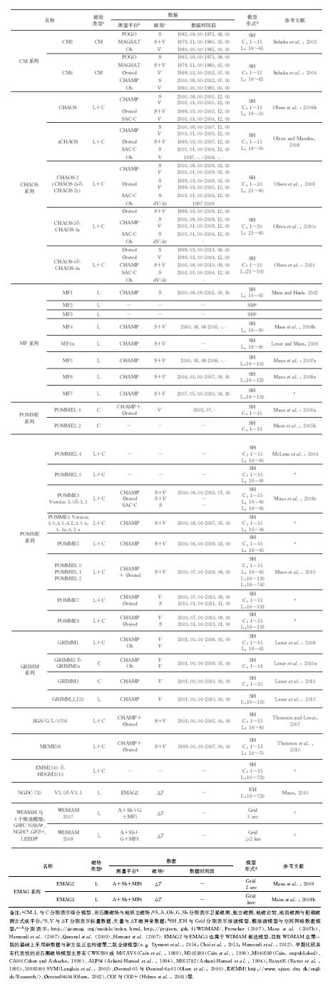
随着卫星技术与磁测技术的快速发展,人类已经发射多颗对地磁场观测卫星(冯彦等,2010; Olsen et al.,2010a; Olsen and Kotsiaros,2011; Olsen and Stolle,2012),如表 1所示.根据发射日期,可以将磁测卫星的发展历程分为三个阶段:早期磁测卫星(20世纪60年代至20世纪末),主要以POGO和MAGSAT卫星为代表;现代磁测卫星(1999年至2009年),以Øersted、SAC-C/Øersted-2、CHAMP卫星为代表;新一代磁测卫星(2010年至今),主要为欧空局(ESA)于2013年11月22日发射升空的Swarm磁测卫星群(Friis-Christensen et al.,2006).目前在筹卫星主要包括Swarm Follow-on、丹麦的类似GOCE重力卫星的磁力梯度测量卫星(Kotsiaros and Olsen,2014)、中国科学院地质与地球物理研究所的中国地磁测量小卫星群计划(5颗子卫星)(Du,2014)以及中国地震局地震预测研究所的中国电磁监测试验卫星(预计将于2016年末发射)(Shen et al.,2014).
|
| 表 1 用于地磁场建模的磁测卫星(Olsen et al.,2010a,b) Table 1 Satellite missions of relevance for geomagnetic field modelling(Olsen et al.,2010a,b) |
由表 1可以看出,磁测卫星的测量精度在不断提高,测量方式由标量测量发展为标量与矢量同时测量,由单颗的卫星发展为多颗的卫星群,卫星轨道设计也更加优化.相比CHAMP卫星而言,欧空局于2013年11月22日发射升空的Swarm卫星群具有独特优势:一方面,卫星携带的标量与矢量磁测仪器精度更高,长约9 m的卫星设置使得磁测仪器受卫星本身磁场的影响较小,卫星的坐标定位与姿态定向更加精准,磁测数据的校正/标定方法更加优化(e.g. Hulot et al.,2013,2015; Hulot,2014; Rother et al.,2013; Workshop on the Calibration and Validation(CAL/VAL)of Swarm Level 1b(L1b)Magnetic Field products,held on the afternoon of June 25 as part of session 6 of the Second Swarm International Science Meeting,http://www.swarm-projektbuero.de/fileadmin/Dokumente/Cal-Val_report_SSM2.pdf);另一方面,该卫星由三颗近极轨的子卫星组成,A(Alpha)与C(Charlie)卫星运行于465 km左右的低高度(4年之后将逐渐降低至~350 km),两者地方时相差6分钟、经度相距约1.4°、南北向相距16~80 km、东西向相距155 km,而B(Bravo)卫星的轨道高度为520 km左右,此卫星群设计实现了在地方时-空间方面的更加全面地采样,因而可以根据时空特征对各个起源的磁场进行更好地提取与研究.尤其是A与C卫星近乎平行的同时测量,其磁场差分数据可以更有效地压制非岩石圈起源的磁场以及较好地提取南半球近南北向的岩石圈磁场(e.g. Maus et al.,2006a; Olsen et al.,2006a; Maus,2014;Olsen et al.,2015).特别是Swarm卫星首次实现了对地磁场进行1小时到数天时间尺度之内变化的全球测量,其时空高覆盖采样、东西方向的差分测量以及优化的数据处理流程(e.g. Olsen et al.,2013)将首次对各种场源的磁场进行较完整地分离.由此观测数据构建的岩石圈磁场将弥补球谐模型60~150阶的“空白”波长段(Friis-Christensen et al.,2006),也有望结合陆地与海洋、航空与高空磁测数据实现全球岩石圈磁场的全波段建模.
目前,Swarm卫星群在轨运行正常,单颗卫星的标量测量在磁场宁静时间段的精度优于0.2 nT(e.g. Olsen and the Swarm SCARF Team,2014).已有数据分析表明,由于卫星受太阳光照射存在阴影区,导致卫星本身存在热梯度,使得卫星自身磁场的改正存在波动,但是Nils Olsen教授在2014年的EGU会议上认为此问题不久即将被解决.Swarm卫星L1b数据首次发布于2014年5月22日,重新处理之后的数据发布于2014年7月14日,相关数据可以通过EAS网站下载(https://earth.esa.int/web/guest/missions/esa-operational-eo-missions/swar m),其数据介绍可以通过ESA网站的数据产品手册与Olsen等(2013)进行查阅.其中,Level-2数据分为两类:Cat-1与Cat-2,前类由SCARF(Satellite Constellation Application and Research Facility)设计好的算法每天自动处理,后者的处理比较精细,详细内容可以参阅Olsen等(2013).
至目前,包含了卫星磁测数据的内源场模型已有CHAOS-4plus_V1~V3(Finlay et al.,2014a; Finlay,2014a)、POMME9(http://geomag.org/models/pomme9.html)、CHAOS-5(Finlay et al.,2014b)、SIFM(Olsen et al.,2015)、IGRF12(http://www.ngdc.noaa.gov/IAGA/vm od/igrf.html)及其候选模型(如WMM2015),单纯利用Swarm卫星磁测数据的内源磁场模型已有Swarm_04c(球谐阶次达1~40阶)、SIFM(Olsen et al.,2015)(球谐阶次达1~70阶).虽然目前利用近14个月的Swarm卫星磁测数据恢复的岩石圈磁场只达70阶,但是已经显示出差分梯度数据在内源磁场建模之中的优势(e.g. Kotsiaros et al.,2015;Sabaka et al.,2015;Olsen et al.,2015),并且与利用CHAMP卫星10年观测数据构建的岩石圈磁场模型之间具有较好的一致性,可靠阶次可达65阶(Olsen et al.,2015).随着磁测数据的日益积累,Swarm卫星磁测数据必将在高分辨率与高精度的全球岩石圈磁场建模方面发挥更加显著的作用.
2 全球岩石圈磁场建模的研究现状与发展方向
2.1 全球岩石圈磁场建模方法与模型
基于COSMOS49卫星磁测数据,Zietz等(1970)与Benkova等(1973)分别绘制了美国境内的卫星磁异常图与纬度±50°范围之内的内源场模型.基于POGO卫星磁测数据,Regan等(1975)绘制了±50°范围之内的岩石圈磁异常图,从此开启了利用卫星调查岩石圈磁场的大门.此后,基于Magsat卫星数据或联合POGO数据,涌现了大批全球性与区域性的岩石圈磁异常图(e.g. Langel et al.,1982a,b; Langel,1990a),Langel和Hinze(1998)对其进行了详细地总结.紧接着,在国际位场研究的十年期间(1999-2009),借助于Øersted1&2与CHMAP卫星磁测数据以及非岩石圈磁场的深入研究与数据处理技术的改进,岩石圈磁场模型的分辨率与精度得到大幅度地提升.表 2即总结了2000年之后国际上发布的具有代表性的全球岩石圈磁场模型及其相关参数.下面从采用的磁测数据、岩石圈磁场建模的整体框架、模型形式与国内相关研究现状四个方面分别进行介绍.
|
|
表 2 2000年以后国际上发布的具有代表性的全球岩石圈磁场/内源地磁场模型 Table 2 Representative global lithospheric magnetic field/internal geomagnetic field models released after the year of 2000 |
1)从采用的磁测数据方面来看,已有全球岩石圈磁场建模主要分为:纯卫星磁测数据的建模,又可以进一步分为利用单一卫星计划的单/多颗磁测数据的建模(如MF系列岩石圈磁场模型与GRIMM系列内源场模型)与利用多个卫星计划的多颗卫星磁测数据的建模(如POMME系列、BGS/G/L/0706与MEME08内源场模型);联合地磁台站数据与卫星数据的建模(如CM系列与CHAOS系列内源场模型);联合地面与船载磁测数据、航空磁测数据与卫星磁测数据的建模,其模型形式主要分为两大类,一是基于数学模型的球谐或椭球谐等模型(如NGDC720 v3p1模型),二是空间节点形式的网格数据(如EMAG3、EMAG2与WDMAM及其候选系列模型).由表 2可以看出,CHAMP卫星的磁测数据在全球岩石圈磁场建模之中发挥了极其重要的作用.
2)若利用单一卫星计划的单/多颗磁测数据,从地磁场建模整个框架而言,岩石圈磁场建模主要分为两种类型:一种是综合法建模(Comprehensive Modelling,CM),比较具有代表性的是CM3~CM5内源场模型(Sabaka et al.,2002,2004,2013,2015);另一种是顺序法建模(Sequential Modelling,SM),大多数建模方法均采用SM方法,如比较经典的是MF系列岩石圈磁场模型(Maus et al.,2002).此两种方法的区别主要在于:前者对地核主磁场与岩石圈磁场内源场、磁层与电离层外源场及其耦合场以及变化外源场引起的内源感应磁场同时进行磁场建模,但是其需要各类场源磁场的先验信息(Olsen et al.,2010b),而后者在于首先尽最大努力挑选受外源场影响最小的数据,然后尽量利用最好的其它场源的磁场模型对严格挑选的数据进行改正,再对改正之后的数据进行适当的沿轨滤波与轨间平衡等精细处理,最后对所得的岩石圈磁场数据进行岩石圈磁场制图或反演建模.此两种方法具有各自的优点与缺点,但是相对而言顺序法在岩石圈磁场建模之中应用更加广泛(e.g. Langel,1993)(表 2).
 |
图 1 Swarm卫星主要荷载及其相对位置与卫星自身磁场分布 (图件来源于:http://smsc.cnes.fr/SWARM/index.htm) Fig. 1 The main load and relative position of Swarm satellite and its magnetic field distribution |
 |
图 2 由Swarm卫星磁测数据获得的2014年2月的主磁场(左上)、2月相对于1月的主磁场变化(右上)、岩石圈磁场径向分量(左下)及其相对于CHAOS4模型(Olsen et al.,2014)的空间差异分布(右下) (图件来源于: http://www.esa.int/Our_Activities/Observing_the_Earth/Swarm与ftp://ftp.space.dtu.dk/pub/nio/Swarm/) Fig. 2 By swarm satellite magnetic data obtained by 2014 February the main magnetic field(left),2 months relative to the main magnetic field changes in January |
3)在对原始磁测数据经过一系列数据挑选、改正及数据处理之后,即可认为得到了岩石圈磁场的观测数据,当然不可避免地依然包含部分噪声与残存的其它场源的干扰,接下来即是利用所得观测数据进行岩石圈磁场建模(Finlay et al.,2010),也就是寻找一种对于岩石圈磁场近似的简化描述(representation),其模型主要分为数值模型、数学模型与物理模型(Schott and Thébault,2011; 徐文耀等,2011a,b):数值模型主要有网格节点数据模型、多项式模型(如幂函数、指数函数、三角函数、样条函数、Taylor多项式等),其不包含任何物理意义,只在于单纯地拟合观测值;数学模型主要有球谐/椭球谐模型、球冠谐/改进球冠谐模型、矩谐模型等,其包含的物理意义在于此种表达满足磁位/磁场的物理性质,例如对于无源场满足拉普拉斯方程以及其随空间的衰减性等;而物理模型体现在对其场源的描述与表达,例如对于地核主磁场的地磁发电机模型等,对于岩石圈磁场,其物理模型即为岩石圈之内岩石的磁性分布,也即磁化强度矢量的空间分布.在国际上,早期由于缺乏对非岩石圈起源磁场的建模研究,主要以制图技术为主(综述参见:Langel and Hinze,1998),现在建模所用的模型函数逐渐由以往随空间位置尺度不变的基函数(如球谐函数等)向具有多尺度性能的基函数方向发展,如球面样条函数(e.g. Shure et al.,1982)、等效源方法(e.g. Langlais et al.,2010; Kother,2014; Kother et al.,2014)、球面小波(e.g. Holschneider et al.,2003; Maier,2003; Mayer and Maier,2006; 王慧琳,2010; 张辉等,2010; 赵磊,2010)、局域化谐函数(e.g. Lesur,2006)、球面Slepian基函数(e.g. Simons et al.,2006; Beggan et al.,2013)、球面滑动的改进球冠谐分析(e.g. Thébault,2006; Thébault et al.,2013)等.
4)对于国内的岩石圈磁场建模工作,早期主要以安振昌、徐文耀、徐元芳与王月华等为代表的一批学者结合MAGSAT卫星数据与地磁台站数据构建了大量的中国及亚洲岩石圈磁场模型和主磁场长期变化模型(e.g. 徐文耀和朱岗崑,1984; An et al.,1992a,b; 王月华,1992; 徐元芳等,1997,2000).最近,Ou等(2013)结合地磁台站数据与CHAMP卫星磁测数据构建了中国及其邻区的岩石圈磁场模型,其空间分辨率达到150 km.冯彦(2011)采用中国地区的长期地磁台站数据构建了中国地区主磁场及其长期变化的Taylor多项式与曲面样条模型,并且与CM4模型进行了对比分析.徐文耀、白春华与康国发等所带领的研究组正在进行基于CHAMP卫星磁测数据的中国地区与中国西南地区的岩石圈磁场或磁异常的区域建模及其分布特征研究工作(狄传芝,2009; e.g. 徐文耀等,2011a,b; 白春华等,2011).安振昌等(2014)对1683年至1949年中国地磁测量、地磁图和地磁模型进行了总结与评述.总体而言,目前国内的岩石圈磁场建模研究主要集中于中国和亚洲地区的区域磁场或局部地区磁场建模方面,而且建模方法主要采用数学模型且模型的空间尺度单一;另外,相比而言,国内在卫星磁测数据的标定/校正(如卫星自身磁场改正与欧拉角的确定和校正等)、数据挑选、外磁场及其感应场与主磁场的改正、以及数据处理技术方面落后于国际水平.但是,由于科学、社会与国家发展的强烈需求(e.g. 张昌达,2003; 骆遥,2013),国内在岩石圈磁场建模方面正在努力接近国际水平.因此,开展全球岩石圈磁场建模相关研究适应国内需求,也可以为中国未来的磁测卫星计划提供参考资料.
2.2 全球岩石圈磁场建模的关键联合地面、海洋、航空、高空与卫星磁测数据进行岩石圈磁场建模是发展的必然,但是基于单纯的卫星磁测数据,全球岩石圈磁场建模的关键在于如下四个方面:
1)实测数据的精细挑选.其目的在于尽量挑选受外源场及其感应场影响最弱的数据,对岩石圈磁场建模至关重要(e.g. Thébault et al.,2012),衡量其影响程度的准则种类繁多,不同的建模者采用的准则及其参数也各有不同,相关综述参见Thomson和Lesur(2007)以及徐文耀(2009),但是最常用的挑选准则主要有:地方时(LT),一般选择夜晚时间段的数据,如22:00-5:00,以减弱电离层的Sq电流体系影响;为了减弱极光电流体系的影响,在中、低磁纬度范围内(如±57°)使用三分量矢量数据而在高纬度与极区(如大于+47°与小于-47°)使用标量数据,不同学者采用的磁纬度范围不同且其重叠区域大小也不相同;Quality flags,用于确定卫星姿态的Star Camera是否正常运行;Lesur等(2008)分析认为磁层活动主要影响水平分量,因而将矢量数据由North/East/Center(NEC)直角坐标系旋转至SM直角坐标系(Solar Magnetic Cartesian Coordinate System)之后只采用垂直分量数据(如Maus et al.,2008);Kp指数,用于衡量全球性地磁活动性,如将Kp指数大于2或前3个小时之内Kp指数的变化大于2的数据剔除;Dst指数,用于衡量赤道环电流的强度,如将|Dst|指数大于或等于20 nT或前3个小时之内|Dst|指数的变化大于或等于10 nT的数据剔除,需要注意的是,此类指数在高纬度与极区可能无法较好地描述地磁活动性,而且Olsen等(2005)发现Dst指数的基线值随时间存在变化,因而之后的数据挑选也侧重于该指数的时变性标准,而且Lesur等(2013)研究发现岩石圈磁场信号的误差水平与外源场的方差和同一经度的轨道个数的比例呈正比,因而更应该根据该比例系数作为数据筛选标准(Thébault et al.,2013);行星际磁场(Interplanetary Magnetic Field,IMF),用于衡量太阳风的活动性;ap指数,用于测量行星尺度的一般磁活动性;根据实测标量数据与矢量数据计算的标量数据之间的差异等标定与检验情况,判断是否采用矢量数据.
2)非岩石圈起源的磁场改正.为了获取岩石圈磁场信号,需要对挑选的磁测数据进行非岩石圈起源的地磁场改正,需要改正的磁场主要包括:主磁场、磁层(e.g. 徐文耀等,2008b)与电离层外源场(e.g. Chulliat et al.,2013)及其耦合场以及变化外源场引起的内源感应磁场(主要由包括海洋与地幔产生)(e.g. Olsen et al.,2010b).而早期由于缺乏对其它起源磁场的研究与建模,一般根据时空特征,如按照地方时(如上升轨与下降轨)、磁纬度、不同分量、不同坐标框架(如SM直角坐标系)、观测高度等进行分类,再采用多项式拟合(e.g. Mayhew,1979)、平均法、高斯或拉普拉斯加权插值法(e.g. Kis and Wittmann,1998,2002)或其它沿轨滤波技术以剔除非岩石圈起源的磁场信号(综述参见:Langel and Hinze,1998; Thébault et al.,2012),例如基于沿轨快速傅里叶变换的高通滤波或Kaiser滤波(e.g. Kaiser,1974),其难点在于如何选取截止波长,往往根据采用先验的岩石圈磁场模型与滤波之后的观测数据进行对比分析、通过试错法确定滤波参数,然而其不可避免地会影响真实的岩石圈信号,在应用时需要小心谨慎.现在主要采用其它场源模型直接进行非岩石圈起源的磁场改正处理.其中,为了避免在此过程中丢失真实的岩石圈磁场信号,提升岩石圈磁场数据的信噪比,往往首先采用先验的岩石圈磁场模型从观测数据之中扣除、然后再处理,最后在处理完成之后再将先验模型数据反添加到处理之后的观测数据之中.在此过程之中,不同建模者采用的岩石圈磁场参考场与剩余数据的处理方法与技术和先后流程也不同.
3)进一步的轨间数据分析与滤波等处理.在进行非岩石圈起源的地磁场改正之后,往往在所得数据之中仍然残留了非岩石圈起源的地磁场以及数据噪声.由于卫星的飞行轨道以及之前数据筛选、沿轨滤波等处理,在相邻轨道之间的观测数据存在系统偏离,但是又缺少垂直于飞行轨道的校正基线数据,因此轨道之间的数据分析及其滤波被大量学者采用,例如轨间相关性分析(Pass-by-Pass Correlation)(e.g. Alsdorf,1991; Alsdorf et al.,1994)、轨间线性回归分析(e.g. Ridgway and Hinze,1986)、上升轨与下降轨之间的交叉分析(Crossover Analysis)(e.g. Taylor and Frawley,1987; Ravat,1989)、轨间平衡算法(e.g. Lesur and Maus,2006; Maus et al.,2006b)与协变球谐分析技术(Covariant Spherical Harmonic Analysis)(e.g. Arkani-Hamed and Strangway,1985; Arkani-Hamed et al.,1994)等.进一步的处理即是高度归一化处理(e.g. Regan,1979; Langel et al.,1984; Ravat et al.,1991),常用方法主要有经验性的磁场衰减规律(e.g. Richmond et al.,2005)、最小二乘配置法(e.g. Goyal et al.,1990)、等效源法(e.g. Mayhew,1979; von Frese et al.,1981)与迭代调和级数法(e.g. Henderson and Cordell,1971; 安玉林和管志宁,1993).最后进行奇异观测点与奇异轨道剔除,一般通过对扣除先验岩石圈磁场模型与滤波之后的残余数据进行统计分析判断是否剔除观测点或者观测轨道数据.为了进一步减少模型误差,发展了后滤波处理技术,简单的例如Hanning滤波(http://geomag.org/models/ngdc720.html),而Lesur等(2013)基于误差分布与卫星轨道相关的假设,采用迭代后处理技术(An iterative post-processing technique)同时建立了岩石圈磁场模型与误差分布.另外,在进行磁场改正之前,由于卫星姿态数据可能存在跳跃,从而引起磁测矢量数据出现间断点(e.g. Mayhew et al.,1985; Langel,1990b),针对此Purucker(1991)提出经验处理方法,目前Rother等(2013)采用更先进的算法以确定欧拉角.
4)基于选择的基函数与处理之后的岩石圈磁场观测数据,进行岩石圈磁场反演建模.其发展方向在于由以往随空间位置尺度不变的基函数(如球谐函数等)向具有多尺度性能的基函数方向发展.另外,对于反演方法,早期主要以最小二乘法为主,且数据拟合差也仅采用单一的范数进行测度,而采用多种类型的范数进行数据拟合差测度(e.g. Morschhauser et al.,2014; Kother et al.,2014)以及充分利用全球地磁台站数据进行外源场校正(e.g. Thomson et al.,2010)与在反演过程之中引入更多的先验信息等是未来发展方向(e.g. Maus and Haak,2002).
2.3 全球岩石圈磁场建模的难点
由前分析可知,用于建模的磁测数据经过了数据挑选、非岩石圈起源的磁场改正以及滤波等处理,使得如何有效地提取岩石圈起源的磁场信号及其最终的岩石圈磁场数据的误差评估成为全球岩石圈磁场建模的难点,主要表现在如下几个方面:
1)由于主磁场及外源场等的干扰与混叠,造成岩石圈磁场长波长成分缺失(如球谐模型的1至12~20阶),这也是岩石圈磁场往往被称为岩石圈磁异常场的原因.解决该问题的方法主要为:
(1)卫星观测数据在地方时与空间上的积累.一方面,基于海量的卫星磁测数据,可以通过精细挑选得到受外源场影响最弱的数据集,以用于最终的岩石圈磁场建模;另一方面,各个起源的地磁场一般具有不同的时空尺度特征,利用该时空特征以及高时-空采样数据可以有助于岩石圈磁场信号的分析与提取(e.g. Kunagu et al.,2013).
(2)联合地面、海洋、航空、高空与卫星观测数据以及地磁台站数据.由于地面、海洋与航空磁测数据受外源场的影响相比卫星数据较弱,而且对于岩石圈磁场更加敏感,因此联合多种观测数据进行联合反演或作为参考岩石圈磁场模型用于卫星磁测数据处理有助于减弱非岩石圈磁场的干扰.
(3)非岩石圈起源磁场模型的改进.各个起源的磁场模型与物理机制在相互迭代之中不断引入各自的最新观测数据与约束信息而不断完善,例如对于地核主磁场,地核流体模型的约束可以较好地改善地核主磁场的长期变化与加速度变化(e.g. Lesur et al.,2010b).
(4)基于地质与其它地球物理资料的正演模拟分析(e.g. Meyer et al.,1983; Hahn et al.,1984; Counil et al.,1989; Cohen et al.,1991; Hemant and Maus,2005; Masterton et al.,2013)以及基于岩石圈磁性分布假设的统计分析(e.g. Jackson,1990; Voorhies et al.,2002),尤其是理论频谱分析可为缺失的磁场分布提供约束(Thébault and Vervelidou,2015).此类正演模拟结果可以对以往缺失的岩石圈长波长分布形成初步认识(e.g. Meyer et al.,1985),并且可以用于估计岩石圈磁场感应磁化部分随时间的变化情况(e.g. Thébault et al.,2009)以及揭示小尺度的地核主磁场变化(e.g. Hulot et al.,2009).同时,基于已有的岩石圈磁性分布信息,进行全球岩石圈磁场约束反演建模是未来的一个发展方向.
(5)地磁场观测方式的改进,例如磁力梯度测量(Kotsiaros and Olsen,2014)以及Swarm卫星的东西方向差分梯度测量(e.g. Olsen et al.,2015)以及基于沿轨与轨间差分的梯度数据(e.g. Purucker et al.,2007; Kotsiaros et al.,2015; Sabaka et al.,2015),将有效压制外源场以及长波长的影响.对不同梯度分量进行岩石圈磁场分布与波长范围的敏感度分析,将不同分量合理组合,将有助于未来利用磁力梯度数据进行高分辨率与高精度岩石圈磁场建模研究.
2)磁测数据滤波等处理技术.前已述及,在进行非岩石圈起源的磁场改正之后,磁测数据不可避免地依然含有主磁场及外源场等的干扰,针对此也已经发展了多种滤波方法(参见2.2节),但是均假设误差与卫星轨道相关,所以在滤波的同时也不可避免地滤掉了部分岩石圈磁场信号,尤其是南半球南北向的岩石圈磁场(e.g. Purucker et al.,1997).因此为了避免过多损失有用信号,往往在滤波之前,利用已有较好的岩石圈磁场参考模型从观测数据之中扣除,再进行滤波等处理.总之,滤波等处理对于岩石圈磁场建模至关重要,而其关键在于对非岩石圈起源磁场的时空特征的认知.
3)建模误差与模型可靠性分析技术.对于最终建模的岩石圈磁测数据误差的认知与评估,是岩石圈磁场建模及其可靠性评估的重要方面,也一直是岩石圈磁场建模的难点(e.g. Langel et al.,1989; Langel,1991; Jackson,1990; Rygaard-Hjalsted et al.,1997; Holme et al.,2003; Lowes and Olsen,2004; Fox Maule,2005; Finlay,2014b).Langel(1993)曾说“若一个模型不能够同时提供合理的误差分析,那么建模者是有罪责的”.数据误差主要包括卫星磁测数据误差(主要指磁测仪器的测量误差、定位与定向误差、标定与校正误差等)、建模误差(主要指模型的截断误差、边界误差与舍入误差)(e.g. 徐文耀等,2011b; Schachtschneider et al.,2012)以及系统误差(主要指非岩石圈起源的磁场改正误差等).对于卫星高度的地核主磁场建模,岩石圈起源的中短波长磁场信号可以被视为不相关的高斯噪声,但是长波长成分显示是相关的,如Jackson(1990)与Rygaard-Hjalsted等(1997)研究表明岩石圈磁场在15°~20°范围之内是相关的;岩石圈磁场的理论球谐谱可为主磁场建模提供待求解系数的协方差矩阵信息(Thébault and Vervelidou,2015).而对于岩石圈磁场建模,其数据误差的评估难度更大.一方面,Fox Maule(2005)采用Variogram技术(e.g. Chilés and Delfiner,1999; Wackernagel,2003)对剩余岩石圈磁场数据进行了统计分析,以构建数据协方差矩阵;另一方面,岩石圈磁场模型之间、黄昏组与黎明组之间的对比与相关性分析(包括球谐域与空间域)(e.g. Ravat et al.,1995; Langel,1990)以及球谐谱分析是经典的分析方法,而与已有地质和地球物理资料的相关度统计分析(e.g. Hemant and Maus,2003; Maus et al.,2008),是一种粗略地整体评估岩石圈磁场模型可靠性比较独立的方法.总之,此类方法只能对模型进行整体性评估或误差空间分布的近似分析,而对于误差空间分布的精确分析目前尚无法获得,其根本原因即在于地磁场本身的复杂性,因而无法对各个起源的磁场进行完整与彻底地分离.
3等效源方法的研究现状与发展方向
3.1等效源方法的研究现状
目前,大多数全球岩石圈磁场模型均采用球谐函数形式,旨在对空间磁场的近似表达以及对磁场物理特征的刻画,而等效源方法是一种传统的基于岩石圈物理模型反演的建模方法,其精髓在于通过构建岩石圈磁化强度矢量分布的“等效”场源模型完成对岩石圈磁场的近似表达.该“等效源”思想最早由Dampney(1969)提出,之后被大量学者用于重、磁勘探数据的插值(e.g. Cordell,1992; Mendonça and Silva,1994)、向上或向下延拓(e.g. Emilia,1973; Hansen and Miyazaki,1984; Li and Oldenburg,2010)、化极(e.g. Silva,1986; Leão and Silva,1989; Guspí and Novara,2009)等处理.
Mayhew(1979)首次将其应用于基于球坐标系的区域或全球卫星磁测数据的处理与解释之中.该方法具备如下独特的优势(e.g. Langlais et al.,2010):1)在拟合观测数据反演等效源分布的同时,可以提供一个岩石圈磁场模型,而构建的等效源分布有利于岩石圈地球物理与地质解释(e.g. Mayhew et al.,1980; Mayhew,1982a,b,1985; 徐元芳等,1997,2000);2)具备空间——波数域局域化功能;3)在保证正演精度的前提下可以不受数据类型以及观测数据空间位置的限制;4)可以用于岩石圈磁测数据的转换处理,如曲化平或高度归一化(e.g. Ravat et al.,1995; Purucker et al.,2000)、标量数据向矢量数据的转换(e.g. Purucker,1990)、导数计算(e.g. 邹新民等,1996)、向下延拓(e.g. Achache et al.,1987; Whaler,1994)、化向地磁极(e.g. Langel,1990; Arkani-Hamed and Urquhart,1990)与假重力异常计算(e.g. 邹新民等,1996)等;5)可以用于估算岩石圈磁性底界面的深度起伏( e.g. Fox Maule,2005; Purucker et al.,2002; Rajaram et al.,2009);6)对于岩石圈磁场建模而言,其另一个独特的优势即在于较易引入岩石圈磁性分布的已知先验信息.因而,等效源方法被广泛用于卫星磁测数据的处理、岩石圈磁场建模与地质解释等诸多方面(e.g. von Frese et al.,1981; Purucker et al.,2000; Asgharzadeh et al.,2008; Kother et al.,2014; Kother,2014; Dyment et al.,2014).
但是,在等效源方法发展初期,面临如下限制因素(e.g. Langlais et al.,2010; 徐文耀等,2011a):主偶极磁场作为岩石圈磁化方向的假设条件;岩石圈物理模型受限于磁偶极子分布;等效源的数量、位置与强度的假设具有人为性,反演过程不可避免地存在多解性问题;其未知参数相对于球谐函数建模方法至少提升1倍,而且计算速度较慢.随后,国内外学者对等效源方法进行了改进(相关综述参见:Purucker and Whaler,2007; 杜劲松,2014).在重、磁勘探领域, Leão和Silva(1989)最早引入滑动窗口以减少反演计算量,Li和Oldenburg(2010)采用小波技术对反演核矩阵进行压缩以减少核矩阵存储量,Barnes和Lumley(2011)对等效源进行分组、构建稀疏矩阵以减少存储量与计算量,Oliveira等(2013)采用多项式描述窗口之内的等效源分布以减少反演参数.而在基于球坐标的全球卫星磁测数据处理与建模方面,以Whaler(1994),Whaler和Langel(1996)为代表,考虑剩余磁化效应,将该方法发展为直接反演岩石圈的磁化强度矢量分布,被用于地球、月球与火星等行星的岩石圈磁性与磁场建模(Arkani-Hamed,2002; Langlais et al.,2004; Whaler and Purucker,2005; Chiao et al.,2006; Carley et al.,2012),在理论上完全消除了主偶极磁场作为岩石圈磁化方向的假设条件.Whaler和Langel(1996)与Shure等(1982)改进等效源模型空间分布,即磁偶极源的分布不再按等间隔经纬度网格节点排列而是按场源与观测点之间的距离由近至远呈由密至稀的分布形式(Depleted basis).此外,Covington(1993)与Fox Maule等(2005)采用了球面等面积六面体剖分技术,而Stockmann等(2009)采用了球面三角剖分技术.Kim等(2013)则用于卫星磁测数据与航空磁测数据的岩石圈磁场联合建模.面对大量计算与低效性缺陷,Langel等(1984)与Ridgway和Hinze(1986)采用分区反演、反演之后再融合的方法,但是不可避免地存在边界效应;Olivier等(1982)提出“bootstrap inversion”方法,主要依据位场叠加性,将一个分区反演的拟合残差作为另一区块的反演数据,von Frese等(1988)对其进行了扩展;而Purucker等(1996)提出根据磁场水平衰减性对反演核矩阵进行稀疏性存储以及共轭梯度优化算法,使得计算效率大幅度提升.
在低磁纬度地区,反演不稳定而出现振荡现象,Mayhew(1979,1980)最初采用全部增大偶极源间距的方式或者采用低纬度较大而高纬度较小的偶极源间距方式以获得稳定解,Basavaiah等(1989)认为该不稳定性是由磁异常的幅值或能量本身随纬度存在变化而引起,Langel等(1984)、Achache等(1987)与Purucker(1990)采用主成分分析或奇异值分解方法以获得稳定解, Lötter(1987)与von Frese等(1988)采用了脊回法(ridge regression),Purucker等(1998)在反演过程之中引入大量地震、地质与岩石磁学资料至初始模型,而Whaler等(1994,1996,2005)则对模型复杂度(即正则化稳定项)进行约束,但是由于仅采用全球统一的最小模型使得反演的磁化强度振幅与方向变化剧烈,而与实际情况差异较大(Whaler,2007).
此外,相对于空间域方法,Arkani-Hamed和Strangway(1985),Arkani-Hamed和Dyment(1996)提出与发展了球谐域的等效源方法.进一步地,Gubbins等(2011)引入矢量球谐分析方法,可以将岩石圈磁场近似转换得到岩石圈单层磁化强度矢量分布,但是其假设条件是磁性层相比于观测数据高度而言视为磁性面.国内学者安玉林和管志宁(1993)也讨论了球谐域的转换方法,但仅适用于径向磁化的情形.总之,球谐域方法的优点在于计算速度较快,但是空间域方法相比球谐域方法灵活性更高、比较容易引入约束信息,也可以处理更加复杂的情况(如椭球壳而不是球壳分布以及磁性层顶底界面起伏等).
3.2等效源方法的发展方向
尽管大量学者对空间域等效源方法进行了不同程度的改进,但是依然存在如下局限性.传统等效源方法的“等效性”不强调岩石圈物理模型的合理性而只关注对磁测数据的单纯拟合.虽然物理模型预测的岩石圈磁场能够拟合观测数据,但是在进一步地转换处理(如延拓与化极等)时则会存在较大误差.但是,从理论上而言,如果反演构建的岩石圈物理模型与实际情况更加接近,则与之对应的岩石圈磁场也将更加真实与可靠(e.g. Regan,1979).基于此思想,等效源方法在岩石圈磁场建模方面的发展方向在于:
1)岩石圈磁性基本模型的改进:一是,岩石圈磁化强度矢量分布由球面磁偶极源分布发展为椭球面棱柱体分布;二是,将考虑岩石圈磁性层的顶界面(如沉积层底界面)与底界面(如Moho面或居里等温面等)的空间变化,虽然对于卫星高度而言,磁性层位置与层厚的变化对建模影响很弱,但是在曲化平、化极与向下延拓等转换处理时,岩石圈磁场的畸变性将会增大;三是,由单层模型发展为多层或三维模型(e.g. Du et al.,2013,2014; 杜劲松,2014),借助于多尺度反演、稀疏核矩阵法(e.g. Purucker et al.,1996; Achache et al.,1987)与并行计算等先进技术,基于数据多尺度分解的多层等效源方法具备可行性,对于岩石圈磁场建模、转换处理及其地质解释也将发挥重要的作用.
2)正演方法的改进:以往的正演方法均基于磁偶极源方法,对于卫星高度的磁位与磁场矢量,其正演精度能够满足要求,但是对于磁力梯度其计算误差较大,而且在向下延拓时,磁偶极源的正演误差会大幅度增加(e.g. 杜劲松,2014).因此,发展正演精度较高的基于球坐标系的磁位、磁场及磁力梯度正演方法非常迫切,如高斯-勒让德数值积分法(e.g. von Frese et al.,1981; Asgharzadeh et al.,2008; 杜劲松,2014; Du et al.,2015).
3)反演方法的改进:一是,由以往的矢量磁化强度三分量反演发展为磁化强度矢量的振幅与方向反演,如此有利于引入磁化方向等先验信息;二是,以往的数据拟合差与模型复杂度的测度函数种类单一而且全球无变化,如Whaler(2007)采用全球不变的L1范数,导致反演的大陆地区磁化方向变化与实际磁化场的方向变化差异较大,而经验表明在海洋与大陆地区,可能适合采用不同的测度函数,发展混合范数(Farquharson and Oldenburg,1998)与自适应混合范数(Sun and Li,2014)具有较好的应用前景;三是,为了使得等效源的横向分布更加可靠,合理地引入先验地质信息(如洋壳年龄分布信息等),将有助于提高岩石圈磁场模型的可靠性.
4 结 论
4.1 地磁观测与地磁场建模是地磁学研究和应用的重要内容之一,而具有独特优势的卫星磁测为全球岩石圈磁场建模提供了有效的途径,对导航、通信、地球物理、大地构造与地球动力学等具有重要意义.本文首先总结了已有的地磁测量卫星,重点地介绍了Swarm卫星的优势与最新动态.其次系统总结了全球岩石圈磁场建模方法与已有的磁场模型,并且指出全球岩石圈磁场建模的关键、难点与发展趋势.最后较详细地介绍了等效源方法在卫星磁测数据处理、岩石圈磁场建模及其地学解释方面的发展历程与研究现状,并且对等效源方法在卫星磁测数据处理、岩石圈磁场建模与地质解释方面的应用前景进行了分析. 4.2 论文旨在为国内的相关学者们对于全球岩石圈磁场建模的发展动态与趋势形成一定程度地了解,也为中国未来的地磁测量卫星计划提供参考资料.通过全文分析可知:一方面,我国即将发射地球磁测卫星,因此在卫星磁测数据的标定/校正、数据挑选、外磁场及其感应场与主磁场的改正、以及数据处理技术方面应该加大研究力度,更为重要的是,国内偏重于基于地磁台站数据与卫星数据进行局部与区域性主磁场与岩石圈磁场建模,需要将局部、区域性扩展至全球性;另一方面,中国及其毗邻海区1:500万航空磁力异常图已于2003年10月出版,然而现有的全球WDMAM模型在中国及其邻区存在大面积的数据空白区(尤其是西部地区),期盼相关部门采取相应措施或开展区域或全球岩石圈磁场建模工作,以更好地为全球地磁场相关科学研究作出贡献. 致 谢 感谢中国地质大学(武汉)地球物理与空间信息学院的孙石达在论文文字方面的检查以及审稿专家的指导与帮助.
| [1] | Achache J, Abtout A, Le Mouël J L. 1987. The downward continuation of Magsat crustal anomaly field over Southeast Asia [J]. Journal of Geophysical Research, 92(B11): 11584-11596. |
| [2] | Achache J, Cohen Y, Unal G. 1991. The French program of circumterrestrial magnetic surveys using stratospheric balloons [J]. EOS Transactions of the American Geophysical Union, 72(9): 97-101. |
| [3] | Alsdorf D, Nelson D. 1999. Tibetan satellite magnetic low: Evidence for widespread melt in the Tibetan crust? [J]. Geology, 27(10): 943-946. |
| [4] | Alsdorf D E. 1991. Statistical processing of Magsat data for magnetic anomalies of the lithosphere [M. S. thesis]. Columbus: The Ohio State University. |
| [5] | Alsdorf D E, von Frese R R B, Arkani-Hamed J, et al. 1994. Separation of lithospheric, external, and core components of the south polar geomagnetic field at satellite altitudes[J]. Journal of Geophysical Research, 99(B3): 4655-4668. |
| [6] | An Y L, Guan Z N. 1993. Conversion methods of the Magsat anomaly in spherical coordinate system [J]. Geoscience (in Chinese), 7(1): 118-124. |
| [7] | An Z C, Xu Y F, Wang Y H, et al. 1992a. Scalar and vector magnetic anomaly maps for China derived from Magsat data [J]. Chinese Journal of Space Science, 12(2): 123-128. |
| [8] | An Z C, Ma S Z, Tan D H, et al. 1992b. A spherical cap harmonic model of the satellite magnetic anomaly field over China and adjacent areas [J]. Journal of Geomagnetism and Geoelectricity, 44(3): 243-252. |
| [9] | An Z C, Peng F L, Liu S H, et al. 2014. Inspection and study on the geomagnetic survey, charts and models during 1683-1949 in China[J]. Chinese Journal of Geophysics (in Chinese), 57(11): 3795-3803. |
| [10] | Arkani-Hamed J, Strangway D W. 1985. Lateral variations of apparent magnetic susceptibility of lithosphere deduced from Magsat data [J]. Journal of Geophysical Research, 90(B3): 2655-2664. |
| [11] | Arkani-Hamed J, Urquhart W E S. 1990. Reduction to the pole of the North American magnetic anomalies [J]. Geophysics, 55(2): 218-225. |
| [12] | Arkani-Hamed J, Langel R A, Purucker M E. 1994. Scalar magnetic anomaly maps of Earth derived from POGO and Magsat data [J]. Journal of Geophysical Research, 99(B12): 24075-24090. |
| [13] | Arkani-Hamed J, Dyment J. 1996. Magnetic potential and magnetization contrasts of Earth’s lithosphere [J]. Journal of Geophysical Research, 101(B5): 11401-11425. |
| [14] | Arkani-Hamed J. 2002. Magnetization of the martian crust [J]. Journal of Geophysical Research, 107(E5), doi: 10.1029/2001J E001496. |
| [15] | Asgharzadeh M F, von Frese R R B, Kim H R. 2008. Spherical prism magnetic effects by Gauss-Legendre quadrature integration [J]. Geophysical Journal International, 173(1): 315-333. |
| [16] | Bai C H, Kang G F, Gao G M. 2011. Impact of the CHAMP satellite processing scheme on the geomagnetic modelling [C]. //Proceedings of 27th Chinese Geophysical Society (CGS) Annual Meeting. Hefei, China: Press of University of Science and Technology of China, p. 871. |
| [17] | Barnes G, Lumley J. 2011. Processing gravity gradient data [J]. Geophysics, 76(2): 133-147. |
| [18] | Basavaiah N, Rajaram M, Singh B P. 1989. Comments on latitudinal dependence of MAGSAT anomalies in the B field and associated inversion instabilities [J]. Physics of the Earth and Planetary Interiors, 55(1-2): 26-30. |
| [19] | Beggan C D, Saarimäki J, Whaler K A, et al. 2013. Spectral and spatial decomposition of lithospheric magnetic field models using spherical Slepian functions [J]. Geophysical Journal International, 193(1): 136-148. |
| [20] | Benkova N P, Dolginov Sh Sh, Simonenko T N. 1973. Residual geomagnetic field from the satellite cosmos 49 [J]. Journal of Geophysical Research, 78(5): 798-803. |
| [21] | Blakely R G. 1995. Potential Theory in Gravity and Magnetic Applications [M]. Cambridge: Cambridge University Press. |
| [22] | Cain J C, Wang Z G, Kluth C, et al. 1989. Derivation of a geomagnetic model to n=63 [J]. Geophysical Journal International, 97(3): 431-441. |
| [23] | Cain J C, Hulter B, Sandee D. 1990. Numerical experiments in geomagnetic modeling [J]. Journal of Geomagnetism and Geoelectricity, 42(9): 973-987. |
| [24] | Carley R A, Whaler K A, Purucker M E, et al. 2012. Magnetization of the lunar crust [J]. Journal of Geophysical Research, 117: E08001, doi: 10.1029/2011JE003944. |
| [25] | Chiao L Y, Lin J R, Gung Y C. 2006. Crustal magnetization equivalent source model of Mars constructed from a hierarchical multiresolution inversion of the Mars Global Surveyor data [J]. of Geophysical Research, 111: E12010, doi: 10.1029/2006JE002725. |
| [26] | Chilés J P, Delfiner P. 1999. Geostatistics: Modeling Spatial Uncertainty [M]. New York: John Wiley & Sons. |
| [27] | Choi Y, Dyment J, Hamoudi M, et al. 2013. WDMAM version 2: a new global magnetic anomaly map over the oceans [C]. // 12th IAGA Scientific Assembly. Merida, Mexico. |
| [28] | Chulliat A, Vigneron P, Thébault E, et al. 2013. Swarm SCARF dedicated ionospheric field inversion Chain [J]. Earth, Planets and Space, 65(11): 1271-1283. |
| [29] | Cohen Y, Menvielle M, Le Mouel J L. 1986. Magnetic measurements aboard a stratospheric balloon [J]. Physics of the Earth and Planetary Interiors, 44(4): 348-357. |
| [30] | Cohen Y, Achache J. 1990. New global vector magnetic anomaly maps derived from Magsat data [J]. Journal of Geophysical Research, 95(B7): 10783-10800. |
| [31] | Cordell L. 1992. A scattered equivalent-source method for interpretation and gridding of potential-field data in three dimensions [J]. Geophysics, 57(4): 629-636. |
| [32] | Counil J L, Achache J, Cohen Y. 1989. Global long wavelength magnetic signal induced by the ocean/continent susceptibility contrast [J]. IAGA Bulletin, 53: 182. |
| [33] | Counil J L, Cohen Y, Achache J. 1991. The global continent-ocean magnetization contrast [J]. Earth and Planetary Science Letters, 103(1-4): 354-364. |
| [34] | Covington J. 1993. Improvement of equivalent source inversion technique with a more symmetric dipole distribution model [J]. Physics of the Earth and Planetary Interiors, 76(3-4): 199-208. |
| [35] | Dampney C N G. 1969. The equivalent source technique [J]. Geophysics, 34(1): 39-53. |
| [36] | Di C Z. 2009. The study of distribution characteristics about lithospheric magnetic anomaly of satellite observarion in the south-west regions of China (in Chinese) [Master thesis]. Kunming: Yunnan University. |
| [37] | Du A M. 2014. Chinese Geomagnetic Small Multi-satellite Mission [C]. // Third Swarm Science Meeting, IDA Conference Centre in Copenhagen, June 19th to 20th 2014, Abstract Book, p. 5-8. |
| [38] | Du J S, Chen C, Liang Q, et al. 2013. 3-D inversion of the regional magnetic data in spherical coordinates and its preliminary application in Australia [C]. ASEG Extended Abstracts, (1): 1-4. |
| [39] | Du J S. 2014. Study on processing, forward modeling and inversion algorithms of satellite magnetic anomaly data in spherical coordinate system (in Chinese) [Ph. D thesis]. Wuhan: China University of Geosciences. |
| [40] | Du J S, Chen C, Lesur V, et al. 2014. Three dimensional lithospheric magnetization structures beneath Australia derived by inverse modeling of CHAMP satellite magnetic field model [C]. // EGU General Assembly 2014, Geophysical Research Abstracts, Vol. 16, EGU2014-1315-1. Vienna, Austria. |
| [41] | Du J S, Chen C, Lesur V, et al. 2015. Magnetic potential, vector and gradient tensor fields of a tesseroid in a geocentric spherical coordinate system[J]. Geophysical Journal International, 201(3): 1977-2007. |
| [42] | Dyment J, Choi Y, Hamoudi M, et al. 2014. Equivalent magnetization over the World's Ocean and the World Digital Magnetic Anomaly Map [C]. //EGU General Assembly 2014, Geophysical Research Abstracts, Vol. 16, EGU2014-13383. Vienna, Austria. |
| [43] | Emilia D A. 1973. Equivalent sources used as an analytic base for processing total magnetic field profiles [J]. Geophysics, 38(2): 339-348. |
| [44] | Farquharson C G, Oldenburg D W. 1998. Non-linear inversion using general measures of data misfit and model structure [J]. Geophysical Journal International, 134(1): 213-227. |
| [45] | Feng Y, An Z C, Sun H, et al. 2010. Geomagnetic survey satellites [J]. Progress in Geophysics (in Chinese), 25(6): 1947-1958, doi: 10.3969/j.issn.1004-2903.2010.06.009. |
| [46] | Feng Y. 2011. Simulation of lithospheric magnetic field over Chinese mainland (in Chinese) [Ph. D thesis]. Nanjing: Nanjing Agricultural University. |
| [47] | Finlay C C, Maus S, Beggan C D, et al. 2010. International geomagnetic reference field: the eleventh generation [J]. Geophysical Journal International, 183(3): 1216-1230. |
| [48] | Finlay C. 2014a. Use of Swarm data in an update of the CHAOS-4 field model [C]. //Third Swarm Science Meeting, IDA Conference Centre in Copenhagen, June 19th to 20th 2014, Abstract Book, p. 10. |
| [49] | Finlay C. 2014b. Data error covariances for satellite magnetic data [C]. // Third Swarm Science Meeting, IDA Conference Centre in Copenhagen, June 19th to 20th 2014, Abstract Book, p. 33. |
| [50] | Finlay C C, Olsen N, Tøffner-Clausen L. 2014a. Towards CHAOS-5-How can Swarm contribute? [C]. //EGU General Assembly 2014, Geophysical Research Abstracts, Vol. 16, EGU2014-10878, EGU General Assembly 2014. |
| [51] | Finlay C C, Olsen N, and Tøffner-Clausen L. 2014b. Updating the CHAOS series of field models using Swarm data and resulting candidate models for IGRF-12[C]. 2014 AGU Fall Meeting, December 15th to 19 2014, San Francisco, CA, United States. |
| [52] | Fox Maule C, Purucker M E, Olsen N, et al. 2005. Heat flux anomalies in Antarctica revealed by satellite magnetic data [J]. Science, 309(5733): 464-467. |
| [53] | Fox Maule C. 2005. Geophysical interpretation of magnetic field models-Estimation of the geothermal heat flux underneath the ice caps in Antarctica and Greenland from magnetic field models based on satellite magnetic data [Ph. D Thesis]. Denmark: University of Copenhagen. |
| [54] | Friis-Christensen E, Lühr H, Hulot G. 2006. Swarm: A constellation to study the Earth’s magnetic field [J]. Earth, Planets and Space, 58(4): 351-358. |
| [55] | Gao G M, Kang G F, Bai C H, et al. 2013. Distribution of the crustal magnetic anomaly and geological structure in Xinjiang, China [J]. Journal of Asian Earth Sciences, 77: 12-20. |
| [56] | Goyal H K, von Frese R R B, Hinze W J, et al. 1990. Statistical prediction of satellite magnetic anomalies [J]. Geophysical Journal International, 102(1): 101-111. |
| [57] | Gubbins D, Ivers D, Masterton S M, et al. 2011. Analysis of lithospheric magnetization in vector spherical harmonics [J]. Geophysical Journal International, 187(1): 99-117. |
| [58] | Guspí F, Novara I. 2009. Reduction to the pole and transformations of scattered magnetic data using Newtonian equivalent sources [J]. Geophysics, 74(5): L67-L73. |
| [59] | Hahn A, Ahrendt H, Jeyer J, et al. 1984. A model of magnetic sources within the Earth’s crust compatible with the field measured by the satellite Magsat [J]. Geologisches Jahrbuch Reihe A, 75: 125-156. |
| [60] | Hamilton B. 2013. Rapid modelling of the large-scale magnetospheric field from Swarm satellite data [J]. Earth, Planets and Space, 65(11): 1295-1308. |
| [61] | Hamoudi M, Thébault E, Lesur V, et al. 2007. GeoForschungsZentrum Anomaly Magnetic Map (GAMMA): A candidate model for the World Digital Magnetic Anomaly Map [J]. Geochemistry, Geophysics, Geosystems, 8(6): Q06023, doi: 10.1029/2007GC001638. |
| [62] | Hamoudi M, Dyment J, Choi Y, et al. 2012. World Digital Magnetic Anomaly Map (WDMAM) rev. 2: Oceanic Domains [C]. // AGU Fall Meeting, San Francisco, 3-7 December 2012, ePosters: T43D-2710. |
| [63] | Hansen R O, Miyazaki Y. 1984. Continuation of potential fields between arbitrary surfaces [J]. Geophysics, 49(6): 787-795. |
| [64] | Hemant K, Maus S. 2003. A Comparison of Global Lithospheric Field Models Derived from Satellite Magnetic Data [C] // Reigber C, Lühr H, Schwinzer P eds. First CHAMP Mission Results for Gravity, Magnetic and Atmospheric Studies. Berlin, Heidelberg: Springer, 261-268. |
| [65] | Hemant K, Maus S. 2005. Geological modeling of the new CHAMP magnetic anomaly maps using a geographical information system technique [J]. Journal of Geophysical Research, 110; B12103, doi: 10.1029/2005JB00383 7. |
| [66] | Hemant K, Thébault E, Mandea M, et al. 2007. Magnetic anomaly map of the world: merging satellite, airborne, marine and ground-based magnetic data sets [J]. Earth and Planetary Science Letters, 260(1-2): 56-71. |
| [67] | Henderson R G, Cordell L. 1971. Reduction of unevenly spaced potential field data to a horizontal plane by means of finite harmonic series [J]. Geophysics, 36(5): 856-866. |
| [68] | Holme R, Olsen N, Rother M, et al. 2003. CO2-a CHAMP magnetic field model [C] // Reigber C, Lühr H, Schwintzer P eds. First CHAMP Mission Results for Gravity, Magnetic and Atmospheric Studies. Berlin: Springer, 220-225. |
| [69] | Holschneider M, Chambodut A, Mandea M. 2003. From global to regional analysis of the magnetic field on the sphere using wavelet frames [J]. Physics of the Earth and Planetary Interiors, 135(2-3): 107-124. |
| [70] | Hulot G, Olsen N, Thébault E, et al. 2009. Crustal concealing of small-scale core-field secular variation [J]. Geophysical Journal International, 177(2): 361-366. |
| [71] | Hulot G, Finlay C C, Constable C G, et al. 2010. The Magnetic Field of Planet Earth [J]. Space Science Reviews, 152(1-4): 159-222. |
| [72] | Hulot G, Leger J M, Crespo-Grau R, et al. 2013. A proposal to cross-validate ESA’s Swarm Level 1b data with Absolute Scalar Magnetometer experimental vector mode data [C]. // European Space Agency Living Planet Symposium, from 09 to 13 September 2013. Edinburgh, United Kingdom. |
| [73] | Hulot G. 2014. On the possibility of using Swarm’s Absolute Scalar Magnetometer experimental vector field measurements to produce alternative geomagnetic field models and North East Centre vector data [C]. // Third Swarm Science Meeting, IDA Conference Centre in Copenhagen, June 19th to 20th 2014, Abstract Book, 13-66. |
| [74] | Hulot G, Vigneron P, and Léger J, et al. 2015. Swarms absolute magnetometer experimental vector mode, an innovative capavility for space magnetometry[J]. Geophysical Research Letters, 42, doi:10.1002/2014GL062700. |
| [75] | Jackson A. 1990. Accounting for crustal magnetization in models of the core magnetic field [J]. Geophysical Journal International, 103(3): 657-673. |
| [76] | Kaiser J F. 1974. Nonrecursive digital filter design using the Io-sinh window function [C]. // Proceedings of IEEE International Symposium on Circuits and Systems, 20-23. |
| [77] | Kang G F, Gao G M, Bai C H, et al. 2010. Distribution of magnetic anomalies for the CHAMP satellite in China and adjacent areas [J]. Chinese Journal of Geophysics (in Chinese), 53(4): 895-903, doi: 10.3969/j.issn.0001-5733.2010.04.014. |
| [78] | Kang G F, Gao G M, Bai C H, et al. 2012. Characteristics of the crustal magnetic anomaly and regional tectonics in the Qinghai-Tibet Plateau and the adjacent areas [J]. Science China Earth Sciences, 55(6): 1028-1036. |
| [79] | Kang G F, Gao G M, Bai C H, et al. 2013. Study on distribution features of crustal magnetic anomalies around eastern Himalayan syntaxis [J]. Chinese Journal of Geophysics (in Chinese), 56(11): 3877-3886, doi: 10.6038/cjg20131129. |
| [80] | Kim J W, Kim H R, Von Frese R, et al. 2013. Geopotential field anomaly continuation with multi-altitude observations [J]. Tectonophysics, 585: 34-47. |
| [81] | Kis K I, Wittmann G. 1998. Determination of vertical magnetic anomalies and equivalent layer for the European region from the Magsat measurements [J]. Journal of Applied Geophysics, 39(1): 11-24. |
| [82] | Kis K I, Wittmann G. 2002. 3D reduction of satellite magnetic measurements to obtain magnetic anomaly coverage over Europe [J]. Journal of Geodynamics, 33(1-2): 117-129. |
| [83] | Kother L K. 2014. An equivalent source method for modelling the global lithospheric magnetic field [C]. // Third Swarm Science Meeting, IDA Conference Centre in Copenhagen, June 19th to 20th 2014, Abstract Book, 42-43. |
| [84] | Kother L K, Hammer M D, Finlay C C, et al. 2014. An equivalent source method for modelling the global lithospheric magnetic field [C]. EGU General Assembly 2014, Geophysical Research Abstracts, Vol. 16, EGU2014-6673. |
| [85] | Kotsiaros S, Olsen N. 2014. End-to-End simulation study of a full magnetic gradiometry mission [J]. Geophysical Journal International, 196(1): 100-110. |
| [86] | Kotsiaros S, Finlay C C, and Olsen N. 2015. Use of along-track magnetic field differences in lithospheric field modelling[J]. Geophysical Journal International, 200(2): 878-887. |
| [87] | Kunagu P, Balasis G, Lesur V, et al. 2013. Wavelet characterization of external magnetic sources as observed by CHAMP satellite: evidence for unmodelled signals in [JP2]geomagnetic field models [J].Geophysical [JP]Journal International, [JP]192(3): 946-950. |
| [88] | Langel R A, Phillips J D, Horner R J. 1982a. Initial scalar magnetic anomaly map from MAGSAT [J]. Geophysical Research Letters, 9(4): 269-272. |
| [89] | Langel R A, Schnetzler C C, Phillips J D, et al. 1982b. Initial vector magnetic anomaly map from MAGSAT [J]. Geophysical Research Letters, 9(4): 273-276. |
| [90] | Langel R A, Slud V E, Smith P J. 1984. Reduction of satellite magnetic anomaly data [J]. Geophysics, 54: 207-212. |
| [91] | Langel R A, Estes R H, Sabaka T J. 1989. Uncertainty estimates in geomagnetic field modeling [J]. Journal of Geophysical Research, 94(B89): 12281-12299. |
| [92] | Langel R A. 1990a. Study of the crust and mantle using magnetic surveys by Magsat and other satellites [J]. Proceedings of the Indian Academy of Sciences, 99(4): 581-618. |
| [93] | Langel R A. 1990b. Global magnetic anomaly maps derived from POGO spacecraft data [J]. Physics of the Earth and Planetary Interiors, 62(3-4): 208-230. |
| [94] | Langel R A. 1991. Recent progress in estimating uncertainty in geomagnetic field modeling [J]. Geophysical & Astrophysical Fluid Dynamics, 60(1-4): 37-88. |
| [95] | Langel R A. 1993. The use of low altitude satellite data bases for modeling of core and crustal fields and the separation of external and internal fields [J]. Surveys in Geophysics, 14(1): 31-87. |
| [96] | Langel R A, Purucker M, Rajaram M. 1993. The equatorial electrojet and associated currents as seen in Magsat data [J]. Journal of Atmospheric and Terrestrial Physics, 55(9): 1233-1269. |
| [97] | Langel R A and Purucker M E. 1994. Magnetic anomaly maps of Earth derived from POGO and Magsat data[J]. Journal of Geophysical Research, 99(24): 75-90. |
| [98] | Langel R A, Hinze W J. 1998. The Magnetic Field of the Earth’s Lithosphere: The Satellite Perspective [M] Cambridge, U. K.: Cambridge University Press. |
| [99] | Langlais B, Mandea M, Ultré-Guérard P. 2003. High-resolution magnetic field modeling: application to MAGSAT and Ørsted data [J]. Physics of the Earth and Planetary Interiors, 135(2-3): 77-91. |
| [100] | Langlais B, Purucker M E, Mandea M. 2004. Crustal magnetic field of Mars [J]. Journal of Geophysical Research, 109: E02008, doi: 10.1029/2033JE002048. |
| [101] | Langlais B, Lesur V, Purucker M E, et al. 2010. Crustal magnetic fields of terrestrial planets [J]. Space Science Reviews, 152(1-4): 223-249. |
| [102] | Leo J W D, Silva J B C. 1989. Discrete linear transformations of potential field data [J]. Geophysics, 54(4): 497-507. |
| [103] | Lesur V. 2006. Introducing localized constraints in global geomagnetic field modelling [J]. Earth, Planets and Space, 58(4): 477-483. |
| [104] | Lesur V, Maus S. 2006. A global lithospheric magnetic field model with reduced noise level in the Polar Regions [J].Geophysical Research Letters, 33(13): L13304, doi: 10. 1029/2006GL025826. |
| [105] | Lesur V, Wardinski I, Rother M, et al. 2008. GRIMM: the GFZ Reference Internal Magnetic Model based on vector satellite and observatory data [J]. Geophysical Journal International, 173(2): 382-394. |
| [106] | Lesur V, Wardinski I, Hamoudi M, et al. 2010a. The second generation of the GFZ Reference Internal Magnetic Model: GRIMM-2 [J]. Earth, Planets and Space, 62(10): 765-773. |
| [107] | Lesur V, Wardinski I, Asari S, et al. 2010b. Modelling the Earth’s core magnetic field under flow constraints [J]. Earth, Planets and Space, 62(6): 503-516. |
| [108] | Lesur V, Kunagu P, Wardinski I, et al. 2011. Third version of the GFZ Reference Internal Magnetic Model: GRIMM-3 [C]. Geophysical Research Abstracts, EGU General Assembly 2011, Vol. 13, EGU2011-6154. |
| [109] | Lesur V, Rother M, Vervelidou F, et al. 2013. Post-processing scheme for modelling the lithospheric magnetic field [J]. Solid Earth, 4(1): 105-118. |
| [110] | Li Y G, Oldenburg D W. 2010. Rapid construction of equivalent sources using wavelets [J]. Geophysics, 75(3): L51-L59. |
| [111] | Ltter C J. 1987. Stable inversions of Magsat data over the geomagnetic equator by means of ridge regression [J]. J. Geophys., 61: 77-81. |
| [112] | Lowes F J, Olsen N. 2004. A more realistic estimate of the variances and systematic errors in spherical harmonic geomagnetic field models [J]. Geophysical Journal International, 157(3): 1027-1044. |
| [113] | Luo Y. 2013. A huge gap of the lithospheric magnetic field model in the Qinghai-Tibet Plateau — Comment on “Characteristics of the crustal magnetic anomaly and regional tectonics in the Qinghai-Tibet Plateau and the adjacent areas” [J]. Science China Earth Sciences, 56(9): 1623-1626. |
| [114] | Macmillan S, Olsen N. 2013. Observatory data and the Swarm mission [J]. Earth, Planets and Space, 65(11): 1355-1362. |
| [115] | Maier T. 2003. Multiscale geomagnetic field modelling from satellite data: theoretical aspects and numerical applications [D]. Germany: University of Kaiserslautern. |
| [116] | Mandea M, Thébault E. 2007. The changing faces of the earth’s magnetic field: a glance at the magnetic lithospheric field, from local and regional scales to a planetary view [M]. Paris: Commission for Geological Map of the World, 49+1 CD-ROM. |
| [117] | Mandea M, Holschneider M, Lesur, et al. 2010. The Earth’s Magnetic Field at the CHAMP Satellite Epoch[A]. //Flechtner F M et al ed. System Earth via Geodetic-Geophysical Space Techniques[C], Springer Berlin Heidelberg, p. 475-526. |
| [118] | Masterton S M, Gubbins D, Müller R D, et al. 2013. Forward modelling of oceanic lithospheric magnetization [J]. Geophysical Journal International, 192(3): 951-962. |
| [119] | Maus S, Haak V. 2002. Is the long wavelength crustal magnetic field dominated by induced or by remanent magnetisation? [J]. Journal of Indian Geophysical Union, 6(1): 1-5. |
| [120] | Maus S, Rother M, Holme R, et al. 2002. First scalar magnetic anomaly map from CHAMP satellite data indicates weak lithospheric field [J]. Geophysical Research Letters, 29(14), doi: 10.1029/2001GL013685. |
| [121] | Maus S, Lühr H, Balasis G, et al. 2005a. Introducing POMME, the Potsdam Magnetic Model of the Earth [C]. // Reihber C, Lühr H, Schwintzer P, et al ed. Earth Observation with CHAMP: Results From Three Years in Orbit [C]. New York: Springer, 293-298. |
| [122] | Maus S, McLean S, Dater D, et al. 2005b. NGDC/GFZ candidate models for the 10th generation International Geomagnetic Reference Field [J]. Earth, Planets and Space, 57(12): 1151-1156. |
| [123] | Maus S, Lühr H, Purucker M. 2006a. Simulation of the high-degree lithospheric field recovery for the Swarm constellation of satellites [J]. Earth, Planets and Space, 58(4): 397-407. |
| [124] | Maus S, Rother M, Hemant K, et al. 2006b. Earth’s lithospheric magnetic field determined to spherical harmonic degree 90 from CHAMP satellite measurements [J]. Geophysical Journal International, 164(2): 319-330. |
| [125] | Maus S, Rother M, Stolle C, et al. 2006c. Third generation of the Potsdam Magnetic Model of the Earth (POMME) [J]. Geochemistry, Geophysics, Geosystems, 7(7): Q07008, doi: 10. 1029/2006GC001269. |
| [126] | Maus S, Lühr H, Rother M, et al. 2007a. Fifth-generation lithospheric magnetic field model from CHAMP satellite measurements [J]. Geochemistry, Geophysics, Geosystems, 8(5): Q05013, doi: 10.1029/2006GC001521. |
| [127] | Maus S, Sazonova T, Hemant K, et al. 2007b. National geophysical data center candidate for the world digital magnetic anomaly map [J]. Geochemistry, Geophysics, Geosystems, 8(6): Q06017, doi: 10.1029/2007GC001 643. |
| [128] | Maus S, Yin F, Lühr H, et al. 2008a. Resolution of direction of oceanic magnetic lineations by the sixth-generation lithospheric magnetic field model from CHAMP satellite magnetic measurements [J]. Geochemistry, Geophysics, Geosystems, 9(7): Q07021, doi: 10. 1029/2008GC001949. |
| [129] | Maus S, Fairhead J D, Mogren L S, et al. 2008b. EMAG3: A 3-arc-minute resolution global magnetic anomaly grid compiled from satellite, airborne and marine magnetic data [C]. // 2008 SEG Annual Meeting, Document ID: SEG-2008-0764. |
| [130] | Maus S, Barckhausen U, Berkenbosch H, et al. 2009. EMAG2: A 2-arc min resolution Earth Magnetic Anomaly Grid compiled from satellite, airborne, and marine magnetic measurements [J]. Geochemistry, Geophysics, Geosystems, 10(8): Q08005, doi: 10.1029/2009GC002471. |
| [131] | Maus S. 2010. An ellipsoidal harmonic representation of Earth’s lithospheric magnetic field to degree and order 720 [J]. Geochemistry, Geophysics, Geosystems, 11(6): Q06015, doi: 10. 1029/2010GC003026. |
| [132] | Maus S, Manoj C, Rauberg J, et al. 2010. NOAA/NGDC candidate models for the 11th generation International Geomagnetic Reference Field and the concurrent release of the 6th generation Pomme magnetic model [J]. Earth, Planets and Space, 62(10): 729-735. |
| [133] | Maus S. 2014. Crustal magnetic field mapping from CHAMP to Swarm [C]. // Third Swarm Science Meeting, IDA Conference Centre in Copenhagen, June 19th to 20th 2014, Abstract Book, p. 18. |
| [134] | Mayer C, Maier T. 2006. Separating inner and outer Earth’s magnetic field from CHAMP satellite measurements by means of vector scaling functions and wavelets [J]. Geophysical Journal International, 167(3): 1188-1203. |
| [135] | Mayhew M A. 1979. Inversion of satellite magnetic anomaly data [J]. Journal of Geophysics-Zeitschrift fuer Geophysik, 45(2): 119-128. |
| [136] | Mayhew M A, Johnson B D, Langel R A. 1980. An equivalent source model of the satellite-altitude magnetic anomaly field over Australia [J]. Earth and Planetary Science Letters, 51(1): 189-198. |
| [137] | Mayhew M A. 1982a. Application of satellite magnetic anomaly data to Curie isotherm mapping [J]. Journal of Geophysical Research, 87(B6): 4846-4854. |
| [138] | model for the United States derived from satellite altitude magnetic anomalies [J]. Journal of Geophysical Research, 87(B6): 4837-4845. |
| [139] | Mayhew M A. 1985. Curie isotherm surfaces inferred from high-altitude magnetic anomaly data [J]. Journal of Geophysical Research, 90(B3): 2647-2654. |
| [140] | Mayhew M A, Johnson B D, Wasilewski P J. 1985. A review of problems and progress in studies of satellite magnetic anomalies [J]. Journal of Geophysical Research, 90(B3): 2511-2522. |
| [141] | McLean S, Macmillan S, Maus S, et al. 2004. The US/UK world magnetic model for 2005-2010 [R]. NOAA Tech. Rep. NESDIS/NGDC-1, Natl. Oceanic and Atmos. Admin, Silver Spring, Md. |
| [142] | Mendona C A, Silva J B C. 1994. The equivalent data concept applied to the interpolation of potential field data [J]. Geophysics, 59(5): 722-732. |
| [143] | Meyer J, Hufen J H, Siebert M, et al. 1983. Investigations of the internal geomagnetic field by means of a global model of the Earth’s crust [J]. Journal of Geophysics - Zeitschrift fuer Geophysik, 52: 71-84. |
| [144] | Meyer J, Hufen J H, Siebert M, et al. 1985. On the identification of Magsat anomaly charts as crustal part of the internal field [J]. Journal of Geophysical Research, 90(B3): 2537-2542. |
| [145] | Morschhauser A, Lesur V, Grott M. 2014. A spherical harmonic model of the lithospheric magnetic field of Mars [J]. Journal of Geophysical Research, 119(6): 1162-1188, doi: 10.1002/2013JE004555. |
| [146] | Nazarova K A, Sabaka T, Tsvetkov Y, et al. 2004. Large magnetic anomalies over Russia revealed by balloon data [J]. Russian Journal of Earth Sciences, 6(6): 457-460. |
| [147] | Oliveira V C Jr, Barbosa V C F, Uieda L. 2013. Polynomial equivalent layer [J]. Geophysics, 78(1): G1-G13. |
| [148] | Olivier R, Hinze W J, von Frese R R B. 1982. Satellite magnetic anomalies of Africa and Europe[C]. 52nd Ann. Internat. Mtg., Soc. Explor. Geophys., Expanded Abstracts, p. 413-415. |
| [149] | Olsen N, Holme R, Hulot G, et al. 2000. ?rsted Initial Field Model [J]. Geophysical Research Letters, 27(22): 3607-3610. |
| [150] | Olsen N. 2002. A model of the geomagnetic field and its secular variation for epoch 2000 estimated from ?rsted data [J]. Geophysical Journal International, 149(2): 454-462. |
| [151] | Olsen N, the Swarm End-to-End Consortium. 2004. Swarm—End-to-End mission performance simulator study [R]. ESA contract No. 17263/03/NL/CB, DSRI Report 1/2004, Danish Space Research Institute, Copenhagen. |
| [152] | Olsen N, Sabaka T J, Lowes F. 2005. New parameterization of external and induced fields in geomagnetic field modeling, and a candidate model for IGRF 2005 [J]. Earth, Planets and Space, 57(12): 1141-1149. |
| [153] | Olsen N, Haagmans R, Sabaka T J, et al. 2006a. The Swarm End-to-End mission simulator study: A demonstration of separating the various contributions to Earth’s magnetic field using synthetic data [J]. Earth, Planets and Space, 58(4): 359-370. |
| [154] | Olsen N, Lühr H, Sabaka T J, et al. 2006b. CHAOS—a model of Earth’s magnetic field derived from CHAMP, ?rsted, and SAC-C magnetic satellite data [J]. Geophysical Journal International, 166(1): 67-75. |
| [155] | Olsen N, Mandea M. 2008. Rapidly changing flows in the Earth’s core [J]. Nature Geoscience, 1(6): 390-394. |
| [156] | Olsen N, Mandea M, Sabaka T J, et al. 2009. CHAOS-2—A geomagnetic field model derived from one decade of continuous satellite data [J]. Geophysical Journal International, 179(3): 1477-1487. |
| [157] | Olsen N, Hulot G, Sabaka T J. 2010a. Measuring the Earth’s magnetic field from space: Concepts of past, present and future missions [J]. Space Science Reviews, 155(1-4): 65-93. |
| [158] | Olsen N, Hulot G, Sabaka T J. 2010b. Sources of the geomagnetic field and the modern data that enable their investigation [M]. // Freeden W, Nashed M Z, Sonar T eds. Handbook of Geomathematics. Netherlands: Springer, 105-124. |
| [159] | Olsen N, Mandea M, Sabaka T J, et al. 2010c. The CHAOS-3 geomagnetic field model and candidates for the 11th generation IGRF [J]. Earth, Planets and Space, 62(10): 719-727 |
| [160] | Olsen N, Kotsiaros S. 2011. Magnetic satellite missions and data [M]. //Mandea M, Korte M eds. IAGA Special Sopron Book Series, vol. 5, |
| [161] | Geophysical Research, 100(B10): 20111-20136. |
| [162] | Ravat D, Hildenbrand T G, and Roest W. 2003. New way of processing near-surface magnetic data: The utility of the Comprehensive Magnetic Field Model[J]. The Leading Edge, 22: 784-785. |
| [163] | Regan R D, Cain J C, Davis W M. 1975. A global magnetic anomaly map [J]. Journal of Geophysical Research, 80(5): 794-800. |
| [164] | Regan R D. 1979. The reduction and analysis of satellite magnetometer data [J]. Geophysical Surveys, 3(4): 331-349. |
| [165] | Richmond N C, Hood L L, Mitchell D L, et al. 2005. Correlations between magnetic anomalies and surface geology antipodal to lunar impact basins [J]. Journal of Geophysical Research, 110(E5): E05011. |
| [166] | Ridgway J R, Hinze W J. 1986. MAGSAT scalar anomaly map of South America [J]. Geophysics, 51(7): 1472-1479. |
| [167] | Ritter P, Lühr H, Rauberg J. 2013. Determining field-aligned currents with the Swarm constellation mission [J]. Earth, Planets and Space, 65(11): 1285-1294. |
| [168] | Rother M, Lesur V, Schachtschneider R. 2013. An algorithm for deriving core magnetic field models from the Swarm data set [J]. Earth, Planets and Space, 65(11): 1223-1231. |
| [169] | Rygaard-Hjalsted C, Constable C G, Parker R L. 1997. The influence of correlated crustal signals in modelling the main geomagnetic field [J]. Geophysical Journal International, 130(3): 717-726. |
| [170] | Sabaka T J, Olsen N, Langel R A. 2002. A comprehensive model of the quiet-time, near-Earth magnetic field: phase 3 [J]. Geophysical Journal International, 151(1): 32-68. |
| [171] | Sabaka T J, Olsen N, Purucker M E. 2004. Extending comprehensive models of the Earth’s magnetic field with ?rsted and CHAMP data [J]. Geophysical Journal International, 159(2): 521-547. |
| [172] | Sabaka T J, Olsen N. 2006. Enhancing comprehensive inversions using the Swarm constellation [J]. Earth, Planets and Space, 58(4): 371-395. |
| [173] | Sabaka T J, T?ffner-Clausen L, Olsen N. 2013. Use of the Comprehensive Inversion method for Swarm satellite data analysis [J]. Earth, Planets and Space, 65(11): 1201-1222. |
| [174] | Sabaka T, Olsen N, Tyler R, and Kubshinov A. 2015. CM5, a pre-Swarm comprehensive magnetic field model derived from over 12 years of CHAMP, ?rsted, SAC-C and observatory data[J]. Geophysical Journal International, 200: 1596-1626. |
| [175] | Schott J J, Thébault E. 2011. Modelling the Earth’s magnetic field from global to regional scales [M]. // Mandea M, Korte M eds. IAGA Special Sopron Book Series, vol. 5, Geomagnetic Observation and Models. Netherlands: Springer, 229-264. |
| [176] | Schachtschneider R, Holschneider M, Mandea M. 2012. Error distribution in regional modelling of the geomagnetic field [J]. Geophysical Journal International, 191(3): 1015-1024. |
| [177] | Shen X H, Wang L W, Zhang X M, et al. 2014. The Current Status of the 1st Electromagnetism Satellite Mission in China [C]. Geophysical Research Abstracts, Vol. 16, EGU2014-4730. |
| [178] | Shure L, Parker R L, Backus G E. 1982. Harmonic splines for geomagnetic modelling [J]. Physics of the Earth and Planetary Interiors, 28(3): 215-229. |
| [179] | Silva J B C. 1986. Reduction to the pole as an inverse problem and its application to low-altitude anomalies [J]. Geophysics, 51(2): 369-382. |
| [180] | Simons F J, Dahlen F A, Wieczorek M A. 2006. Spatiospectral concentration on a sphere [J]. SIAM Review, 48(3): 504-536. |
| [181] | Stockmann R, Finlay C C, Jackson A. 2009. Imaging Earth’s crustal magnetic field with satellite data: a regularized spherical triangle tessellation approach [J]. Geophysical Journal International, 179(2): 929-944. |
| [182] | Sun J J, Li Y G. 2014. Adaptive Lp inversion for simultaneous recovery of both blocky and smooth features in a geophysical model [J]. Geophysical Journal International, 197(2): 882-899. |
| [183] | Thébault E. 2006. Global lithospheric magnetic field modelling by successive regional analysis [J]. Earth, Planets and Space, 58(4): 485-495. |
| [184] | Thébault E, Hemant K, Hulot G, et al. 2009. On the geographical distribution of induced time-varying crustal magnetic fields [J]. Geophysical Research Letters, 36(1): L01307. |
| [185] | Thébault E, Purucker M, Whaler K A, et al. 2010. The magnetic field of Earth's lithosphere [J]. Space Science Reviews, 155(1-4): 95-127. |
| [186] | Vervelidou F, Lesur V, et al. 2012. The satellite along-track analysis in planetary magnetism [J]. Geophysical Journal International, 188(3): 891-907. |
| [187] | Thébault E, Vigneron P, Maus S, et al. 2013. Swarm SCARF dedicated lithospheric field inversion chain [J]. Earth, Planets and Space, 65(11): 1257-1270. |
| [188] | Thébault E, Vervelidou F. 2015. A theoretical spatial power spectrum of the Earth’s lithospheric magnetic field [J]. Geophysical Journal International, 201(2): 605-620. |
| [189] | Thomson A W P, Lesur V. 2007. An improved geomagnetic data selection algorithm for global geomagnetic field modelling [J]. Geophysical Journal International, 169(3): 951-963. |
| [190] | Thomson A W P, Hamilton B, Macmillan S, et al. 2010. A novel weighting method for satellite magnetic data and a new global magnetic field model [J]. Geophysical Journal International, 181(1): 250-160. |
| [191] | Tohyama F Y, Takahashi T. 1992. Observation of the Geomagnetic Field by Polar Patrol Balloon [J]. Journal Solar Terrestrial Environmental Research in Japan, 16: 60. |
| [192] | Vervelidou F, Thébault E. 2014. A global estimate of the Earth’s magnetic crustal thickness [C]. Geophysical Research Abstracts, EGU General Assembly 2014, Vol. 16, EGU2014-6681-1. von Frese R R B, Hinze W J, Braile L W, et al. 1981. Spherical-Earth gravity and magnetic anomaly modeling by Gauss-Legendre quadrature integration [J]. Journal of Geophysics - Zeitschrift fuer Geophysik, 49(3): 234-242. von Frese R R B, Ravat D N, Hinze W J, et al. 1988. Improved inversion of geopotential field anomalies for lithospheric investigations [J]. Geophysics, 53(3): 375-385. |
| [193] | Voorhies C V, Sabaka T J, Purucker M. 2002. On magnetic spectra of Earth and Mars [J]. Journal of Geophysical Research, 107(E6): 1-1-1-10. |
| [194] | Wackernagel H. 2003. Multivariate Geostatistics [M]. 3rd ed. Berlin: Springer. |
| [195] | Wang H L. 2010. Spherical Spectrum and Wavelet Analysis of Satellite Magnetic Data (in Chinese) [Master thesis]. Wuhan: China University of Geosciences. |
| [196] | Wang Y H. 1992. Rectangular harmonic analysis of Magsat vector magnetic anomaly in China [J]. Chinese Journal of Geophysics (in Chinese), 35(5): 655-660. |
| [197] | Whaler K A. 1994. Downward continuation of Magsat lithospheric anomalies to the Earth’s surface [J]. Geophysical Journal International, 116(2): 267-278. |
| [198] | Whaler K A, Langel R A. 1996. Minimal crustal magnetizations from satellite data [J]. Physics of the Earth and Planetary Interiors, 98(3-4): 303-319. |
| [199] | Whaler K A, Purucker M E. 2005. A spatially continuous magnetization model for Mars [J]. Journal of Geophysical Research, 110: E09001, doi: 10. 1029/2004JE002393. |
| [200] | Whaler K A. 2007. Geomagnetism in the satellite era [J]. Astronomy & Geophysics, 48(2): 2.23-2.29. |
| [201] | Xu W Y, Tschu K K. 1984. A study of the RHA for the geomagnetic field of China and neighbouring region [J]. Chinese Journal of Geophysics (in Chinese), 27(6): 511-522. |
| [202] | Xu W Y, Bai C H, Kang G F. 2008a. Global models of the Earth’s crust magnetic anomalies [J]. Progress in Geophysics (in Chinese), 23(3): 641-651. |
| [203] | Xu W Y, Du A M, Bai C H. 2008b. Magnetic field models of the Earth’s magnetosphere [J]. Progress in Geophysics (in Chinese), 23(1): 14-24. |
| [204] | Xu W Y. 2009. Yesterday, today and tomorrow of geomagnetic indices [J]. Progress in Geophysics (in Chinese), 24(3): 830-841, doi: 10.3969/j.issn.1004-2903.2009.03.002. |
| [205] | Xu W Y, Qu J M, Du A M. 2011a. Geomagnetic field modelling for the globe and a limited region [J]. Progress in Geophysics (in Chinese), 26(2): 398-415, doi: 10.3969/j.issn.1004-2903.2011.02.002. |
| [206] | Xu W Y, Qu J M, Du A M. 2011b. An analysis of errors in geomagnetic field models [J]. Progress in Geophysics (in Chinese), 26(5): 1485-1509, doi: 10.3969/j.issn.1004-2903.2011.05.001. |
| [207] | Xu Y F, Barraclough D R, Kerridge D J. 1997. A crustal magnetization model and curie Isothem [J]. Acta Geophysica Sinica (in Chinese), 40(4): 481-486. |
| [208] | Xu Y F, An Z C, Huang B C, et al. 2000. Distribution of apparent magnetization for Asia [J]. Science in China Series D: Earth Science, 43(6): 654-660. |
| [209] | Study of lithospheric magnetic field: A new subdiscipline of satellite geomagnetism [J]. Geological Science and Technology Information (in Chinese), 20(3): 83-90. |
| [210] | Zhang C D. 2003. The past, present and future of the satellite magnetic survey [J]. Geophysical & Geochemical Exploration (in Chinese), 27(5): 329-332. |
| [211] | Zhang H, Zhao L, Chen L W. 2010. Application of Poisson wavelets on the sphere in modeling global geomagnetic field [J]. Journal of Chinese Inertial Technology (in Chinese), 18(4): 450-454. |
| [212] | Zhao L. 2010. Research on Representation of Geomagnetic Field Using Poisson Wavelet on the Sphere (in Chinese) [Master thesis]. Changsha: National University of Defense Technology. |
| [213] | Zietz I, Andreasen G E, Cain J C. 1970. Magnetic anomalies from satellite magnetometer [J]. Journal of Geophysical Research, 75(20): 4007-4015. |
| [214] | Zou X M, Liu X H, Huang W B. 1996. Analysis of the Osaka — Kobe earthquake of Japan —— Inversion of magnetic anomalies by equivalent point source under a circumstances of spherical coordinate [J]. Journal of Changchun University of Earth Sciences (in Chinese), 26(2): 211-215. |
| [215] | 安玉林, 管志宁. 1993. 地球坐标系内的磁场转换方法[J]. 现代地质, 7(1): 118-124. |
| [216] | 安振昌, 彭丰林, 刘少华, 等. 2014. 1683-1949年中国地磁测量、地磁图和地磁模型的总考评与研究[J]. 地球物理学报, 57(11): 3795-3803. |
| [217] | 白春华, 康国发, 高国明. 2011. CHAMP卫星数据处理方法对地磁场建模的影响[C]. //中国地球物理学会第二十七届年会论文集. 合肥: 中国科学技术大学出版社, p. 871. |
| [218] | 狄传芝. 2009. 中国、西南地区岩石圈卫星磁异常分布特征研究[D]. 昆明: 云南大学. |
| [219] | 杜劲松. 2014. 基于球坐标系的卫星磁异常数据处理与正反演方法研究[D]. 武汉: 中国地质大学(武汉). |
| [220] | 冯彦, 安振昌, 孙涵等. 2010. 地磁测量卫星[J]. 地球物理学进展, 25(6): 1947-1958, doi: 10.3969/j.issn.1004-2903.2010.06.009. |
| [221] | 冯彦. 2011. 中国大陆地区的岩石圈磁场模拟研究[D]. 南京: 南京农业大学. |
| [222] | 康国发, 高国明, 白春华等. 2010. 中国及邻近地区CHAMP卫星磁异常的分布特征[J]. 地球物理学报, 53(4): 895-903, doi: 10.3969/j.issn.0001-5733.2010.04.014. |
| [223] | 康国发, 高国明, 白春华等. 2011. 青藏高原及邻区的地壳磁异常特征与区域构造[J]. 中国科学: 地球科学, 41(11): 1577-1585. |
| [224] | 康国发, 高国明, 白春华等. 2013. 喜马拉雅东构造结周边地区地壳磁异常分布特征研究[J]. 地球物理学报, 56(11): 3877-3886, doi: 10.6038/cjg20131129. |
| [225] | 骆遥. 2013. 青藏高原在岩石圈磁场模型中的巨大空白—同“青藏高原及邻区的地壳磁异常特征与区域构造”作者商榷[J]. 中国科学: 地球科学, 43(8): 1376-1378. |
| [226] | 彭聪. 2013. 中国大陆深层区域构造格架—系列解释之磁场格架[J]. 地球学报, 34(1): 121-125. |
| [227] | 王慧琳. 2010. 卫星磁异常球面谱与小波处理方法研究[D]. 武汉: 中国地质大学(武汉). |
| [228] | 王月华. 1992. MAGSAT卫星矢量磁异常的矩谐分析[J]. 地球物理学报, 35(5): 655-660. |
| [229] | 徐文耀, 朱岗崑. 1984. 我国及邻近地区地磁场的矩谐分析[J]. 地球物理学报, 27(6): 511-522. |
| [230] | 徐文耀, 白春华, 康国发. 2008a. 地壳磁异常的全球模型[J]. 地球物理学进展, 23(3): 641-651. |
| [231] | 徐文耀, 杜爱民, 白春华. 2008b. 地球磁层的磁场模型[J]. 地球物理学进展, 23(1): 14-24. |
| [232] | 徐文耀. 2009. 地磁活动指数的过去、现在和未来[J]. 地球物理学进展, 24(3): 830-841, doi: 10.3969/j.issn.1004-2903.2009.03.002. |
| [233] | 徐文耀, 区家明, 杜爱民. 2011a. 地磁场全球建模和局域建模[J]. 地球物理学进展, 26(2): 398-415, doi: 10.3969/j.issn.1004-2903.2011.02.002. |
| [234] | 徐文耀, 区家明, 杜爱民. 2011b. 地磁场模型误差分析中的几个问题[J]. 地球物理学进展, 26(5): 1485-1509, doi: 10.3969/j.issn.1004-2903.2011.05.001. |
| [235] | 徐元芳, Barraclough D R, Kerridge D J. 1997. 地壳磁化强度模型和居里等温面[J]. 地球物理学报, 40(4): 481-486. |
| [236] | 徐元芳, 安振昌, 黄宝春等. 2000. 亚洲地区视磁化强度分布[J]. 中国科学(D辑), 30(4): 388-392. |
| [237] | 张昌达. 2001. 岩石圈磁场研究——卫星地磁学的一个新分支[J]. 地质科技情报, 20(3): 83-90. |
| [238] | 张昌达. 2003. 卫星磁测的过去-现在-未来[J]. 物探与化探, 27(5): 329-332. |
| [239] | 张辉, 赵磊, 陈龙伟. 2010. 球面泊松小波在全球地磁场建模中的应用[J]. 中国惯性技术学报, 18(4): 450-454. |
| [240] | 赵磊. 2010. 基于球面泊松小波的地磁场表示问题研究[D]. 长沙: 国防科学技术大学. |
| [241] | 邹新民, 刘晓华, 黄文兵. 1996. 关于日本阪神地震的分析——球坐标下磁卫星异常的等效源反演[J]. 长春地质学院学报, 26(2): 211-215. |