 2014, Vol. 29


2. 中国科学院大学, 北京 100049
2. University of Chinese Academy of Sciences, Beijing 100049, China
地震波数值模拟是认识地震波传播规律的重要手段,在研究地球内部结构和实际资料的处理与解释方面均发挥着重要的作用.目前,比较常用的方法有,有限差分法(Alford et al., 1974; Kelly et al., 1976; Graves,1996; 兰海强等,2011; 刘少林等,2013)、伪谱法(Fornberg,1988; Carcione and Wang, 1993; Tessmer and Kosloff, 1994)、有限元法(Kuo et al., 1982; Padovani et al., 1994; Komatitsch et al., 1996; Richter,1996; Zhang et al., 2002)、谱元法(Komatitsch and Vilotte, 1998; Komatitsch and Tromp, 1999,2002a,2002b; Chaljub et al., 2007; 王秀明等,2007; Tromp et al., 2008; 王童奎等,2008; 汪文帅等,2012)、有限体积法(Dormy and Tarantola, 1995)等.有限差分法具有编程简单,计算效率高等特点,但是数值频散严重且难以处理起伏地表和自由边界条件(Virieux, 1984,1986; Lan et al., 2011; Lan and Zhang, 2012).伪谱法(Carcione and Wang, 1993)是一种全局的方法,具有计算精度高和数值频散小的特点,但是在强非均匀介质的边界处会出现计算不稳定的现象,它与有限差分法一样,具有难以处理起伏地表和自由边界条件之不足.经典的有限元法克服了大部分这些缺点(Smith, 1975,1980; Marfurt,1984),可适应于任意复杂的几何模型,能够自然地满足自由边界条件(地表的牵引力为零),但仍为低阶的近似,具有计算量大和占用内存大等缺点.谱元法(Komatitsch and Vilotte, 1998)与有限元法类似,通过采用Gauss-Lobatto-Legendre(GLL)积分以得到对角的质量矩阵提高计算效率,为高阶的有限元法并具有较高的计算精度,但计算量和内存占用量仍然较大.
目前,基于四边形网格的谱元法(即经典的谱元法),它结合了低阶的有限元法的灵活性和谱方法的指数收敛性,因其高精度、高效性、弱频散等优点在地震学中得到了广泛的应用(Komatitsch and Tromp, 2002a,2002b).谱元法通过求解波动方程的弱形式,能够适应起伏的地表保持物性的不连续性,并且能够精确地满足自由边界条件(Seriani et al., 1992; Priolo et al., 1994; Faccioli et al., 1997; Paolucci et al., 1999).在每个单元上,GLL插值节点与积分节点重合,利用[-1,1]上的勒让德正交多项式在GLL点上构造基函数,积分则是基于一维GLL积分的张量积(Komatitsch and Vilotte, 1998).上述特殊的正交多项式和插值节点的选择导致对角的质量矩阵,大大提高计算效率,具有与有限差分一样的高效性,可以在时间上显式递推.然而,由于非等间距的插值节点(向两端集中)的使用,致使经典的谱元法所要求的时间步长更小(相比于等间距网格),导致总的时间步数显著增加(Carcione and Wang, 1993; de Basabe and Sen, 2010; Mazzieri and Rapetti, 2012).由于四边形网格不能够灵活地刻画复杂的几何模型,为了能够较精确地刻画起伏地表,则需要在地表附近加密网格,这进一步使得稳定性条件变得更加苛刻,使得所需的总时间步数大大增加.
为了克服四边形网格不能够灵活刻画复杂几何模型的缺点,许多学者做了大量的工作,力图在谱元法中使用三角形(四面体)单元(Horn and Johnson, 1985; Dubiner,1993; Sherwin and Karniadakis, 1995; Chen and Babuka, 1995,1996; Wingate and Boyd, 1996; Taylor and Wingate, 1998; Hesthaven et al., 1998; Karniadakis and Sherwin, 1999; Hesthaven and Teng, 2000; Bos et al., 2001; Taylor et al., 2007; Briani et al., 2012).类似于四边形网格,三角网格谱元法需要解决插值多项式、插值节点和数值积分三个首要问题.三角网格谱元法使用[-1,1]区间上有限维空间的Koornwinder-Dubiner(KD)正交多项式(Dubiner,1993),共有Nt=(N+1)(N+2)/2个KD多项式,其中N为阶数.不同于经典的谱元法,Nt个有限维的插值多项式并非每个都达到N阶(Komatitsch et al., 2001),仅仅最高阶数达到N.为了利用KD多项式在[-1,1]区间上的正交性质,需要引入坍塌(Karniadakis and Sherwin, 1999; Pasquetti and Rapetti, 2004)坐标变换(collapsed coordinate transform),将参考三角形变换成参考四边形,积分则是在变换后的参考四边形中完成的.然而,这种坐标变换会导致插值节点向三角形的一个顶点集中,而且该顶点成为插值多项式的奇异点.
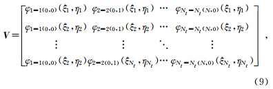
目前,插值节点主要有Fekete点(Taylor and Wingate, 1998; Bos et al., 2001; Taylor et al., 2007; Briani et al., 2012),最小二乘点(Chen and Babuka, 1995,1996)和最小能量电静态点法(Hesthaven,1998; Hesthaven and Teng, 2000).Horn和Bos等证明(Horn and Johnson, 1985; Bos et al., 2001),在三角形的三个边上,Fekete点即为GLL点,并且Fekete点具有最优的插值属性,能够与四边形很好地耦合(Komatitsch et al., 2001).Nt个Fekete插值点被定义为使广义范德蒙德矩阵V的行列式 V 获得最大值的点集(Taylor and Wingate, 1998),其中V的元素为vij=φj(zi),zi为Nt个Fekete点.Fekete点不依赖于多项式的选取,多项式的变化仅仅导致 V 的变化,差异仅为一个常数.在计算这些Fekete点的过程中,力图使 V 获得最大化,以避免矩阵V奇异(Taylor and Wingate, 1998).插值节点的选取至关重要,选取不好会导致数值解振荡(Komatitsch et al., 2001).Pasquetti等人的研究表明(Pasquetti and Rapetti, 2004),三角网格谱元法的条件数随阶数的增长速度远比经典的谱元法快.通常,Fekete点仅仅在低阶情况下有解析表达式,高阶情况下需要通过最优化的方法获取数值解(Taylor and Wingate, 1998; Bos et al., 2001; Taylor et al., 2007; Briani et al., 2012).本文使用的Fekete点来自Briani等人的工作(Briani et al., 2012)(http://www.math.unipd.it/~alvise/sets. html).
为了获取对角的质量矩阵,需要在上述多项式的基础上构造基函数φj(xi),使其具有拉格朗日性质,即φj(xi)=δij.然而,这样的基函数纯粹是为了插值近似构建的,而并非为积分而精确设计的,因此会导致计算精度的下降(Komatitsch et al., 2001).值得指出的是,当插值阶数高于8阶时,积分权重出现负值,这导致计算不稳定(Wingate and Boyd, 1996).特殊地,当插值阶数为2时,对应于三角形顶点的积分权重为0,产生不可逆的质量矩阵,导致二阶的三角网格谱元法不可用.
在计算量方面,Komatitsch等在简单模型中将三角网格谱元法与经典的谱元法做了对比研究(Komatitsch et al., 2001).在每个单元上单个导数的计算,经典的谱元法需要2N+1次浮点操作,而三角网格谱元法却需要(N+1)(N+2)-1次浮点操作,两者的计算量的比值约为N/2.可见,随着阶数的增加,三角网格谱元法的计算量将成倍增加.然而,相比于四边形网格,三角形网格具有更好的灵活性,因此在谱元法中使用三角形网格是有必要的(Pasquetti and Rapetti, 2004,2006,2010; Komatitsch et al., 2001).
本文对三角网格谱元法的基本原理和一些细节问题进行详细地论述,并引入压缩存储行(CSR)格式对谱元法的刚度矩阵进行稀疏存储(Peter,1989; Barrett et al., 1994; Kelley,1995; Saad,2000),以减少计算量并节省内存;对时间离散采用保能量的Newmark算法(Newmark,1959; Kane et al., 1999; West et al., 1999; Krysl and Endres, 2004)以提高其计算精度;将高效的PML吸收边界条件(Chew and Liu, 1996; Collino and Tsogka, 2001; Komatitsch and Tromp, 2003; Martin et al., 2008; 刘有山等, 2012,2013)以变分的形式综合到弹性波动方程的弱形式中以压制来自人工边界的虚假反射波.用拉梅问题(Khun,1985)对显式有限元法(刘有山等,2013)、经典的谱元法和三角网格谱元法的计算精度、计算效率、内存使用量等方面进行对比研究,并验证PML吸收边界条件(刘有山等,2013)的有效性.最后,在起伏地表模型中,就上述三个方面将三角网格谱元法与显式有限元法进行进一步的对比研究.
1 弹性波动方程的弱形式
二维弹性波动方程为

初始条件为
对(1)式的两端乘以虚位移在求解区域进行积分,并利用分部积分可以得到相应的波动方程的弱形式(Komatitsch and Vilotte, 1998)为
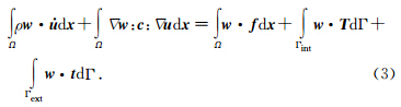
在地震波场数值模拟中,Γint,Γext分别为自由边界条件和人工边界条件;在自由边界条件上,外力 T =σ· n 为常数0;在人工边界条件上需要特殊处理以压制来自人工边界的虚假反射波(刘有山等,2013).
离散后的弹性波动方程可以形成如下的常微分方程组:

2 三角网格谱元法
与有限元法类似,谱元法需要将整个计算区域剖分成Nel个互不重叠的有限个单元Ωe,并在每个单元上用局部的多项式逼近未知函数.
2.1 三角网格谱元法的映射关系
为了实现单元上的数值积分,需要将每个单元Ωe通过可逆变换Fe:Ωe→Λ将其映射到标准区域Λ.不同于经典的谱元法,三角网格谱元法的数值积分,首先将物理区域(图 1a)通过可逆映射将其变换到单位三角形参考区域(即边长为1的等腰直角三角形,见图 1b).由于三角网格谱元法的基函数是在[-1,1]区间上正交的,为了实现单元上的数值积分还需要通过坍塌坐标变换将三角形参考区域(图 1b)进一步映射到[-1,1]2的四边形参考区域(图 1c).
 | 图 1 三角网格谱元法的映射关系示意图
(a)物理区域;(b)三角形参考区域;(c)四边形参考区域.
Fig. 1 The relationship between the physical
element and the reference element for the SEM based on triangular elements(TSEM) (a)The physical domain;(b)The triangular reference domain;(c)The quadrilateral domain. |
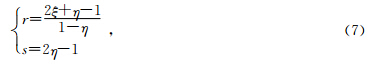
物理区域与参考区域之间的可逆映射关系为
2.2 三角网格谱元法的插值多项式及其积分权重
为了能够在每个单元上用采样点处的波场值来近似局部波场,需要以这些采样点为节点选取一定的多项式逼近未知的波场值.在三角网格谱元法中,插值基函数是基于KD正交多项式构建的,公式为
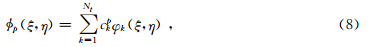
 -1)(1-η)i为KD正交多项式(Komatitsch and Tromp, 2001; Pasquetti and Rapetti, 2004,2006),0≤i,j≤N,且0≤i+j≤N,共有Nt=(N+1)(N+2)/2个,N为阶数.为了书写上的方便,简记
 这里k(i,j)=i×(i+1)/2+j+1;Jα,βi(ξ)为带参数 α,β 的雅可比多项式,J0,0i(ξ)即为i阶的勒让德多项式,Jα,βi(ξ)可以通过递推公式计算(Canuto and Hussaini et al.,2007),其中η=1为坍塌坐标变换引入的奇异点.cpk是正交系数,为广义范德蒙德矩阵V的逆矩阵的第p列.这里,φj(ξi,ηi)为KD正交多项式,φj(ξi,ηi)为基函数.可以证明,KD多项式是在区间[-1,1]上相互正交(Canuto and Hussaini et al.,2007).
广义范德蒙德矩阵为
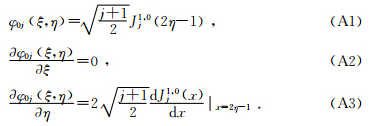
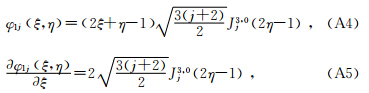
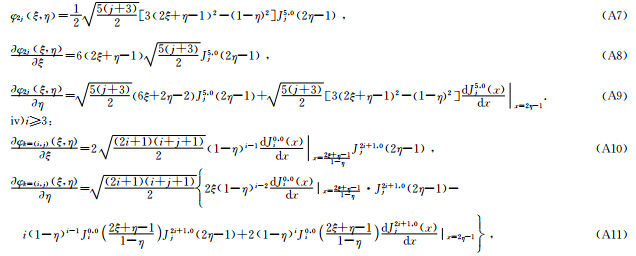
从KD多项式的表达式可见,(ξ,η)=(0,1)为其奇异点,其一阶导数需要分为4类进行分别讨论,详见附录A.
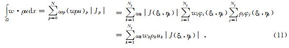
每个单元上的积分通过数值积分来完成.对于上述的基函数,相应的积分权重为

2.3 三角网格谱元法的数值积分
与经典的谱元法类似,通过构造上述的基函数和插值节点,利用重合的插值节点和积分节点性质形成对角的质量矩阵. 三角网格谱元法的对角质量矩阵为
对于刚度矩阵,这里以 为例:
为例:
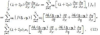
可见,相比于经典的谱元法,三角网格谱元法的刚度矩阵是相对稠密,其计算量约为经典谱元法的N/2倍(Komatitsch et al., 2001).
2.4 PML吸收边界条件
在目前发展起来的众多边界条件中,以PML边界条件的吸收性能较好.为此,本文采用如下的吸收边界条件,并以变分形式应用到三角网格谱元法中,相应的变分形式请详见文献(刘有山等,2013).

3 数值算例
3.1 PML边界条件有效性验证
为了验证本文的PML边界条件的有效性,分别用Sarma边界条件(Sarma and Mallick et al., 1999)和PML边界条件,采用7阶的三角网格谱元法进行波场模拟.模型尺寸为2000 m × 1000 m的均匀介质;纵波速度2000 m/s,横波速度为1150 m/s,瑞雷面波的速度为1058 m/s;密度为2000 kg/m3.震源为10 Hz的雷克子波(垂向集中力源),位于点(1000 m,-50 m)处.网格尺寸为25 m(等腰直角三角形的腰长),PML吸收层厚度为50 m(仅两个谱单元),R取0.001.
图 2为1.0 s时刻的垂直位移分量的波场快照图,其中图 2a为经典的Sarma边界条件的结果,图 2b为本文的PML边界条件的结果.可见,图 2a中存在明显的边界虚假反射波.图 3为(1800 m,0 m)处的水平和垂直分量的地震记录,可以看到本文的PML边界条件取得较好的吸收效果,而Sarma边界条件存在严重的边界虚假反射波.从图 3a可见,Sarma边界条件导致面波的数值解存在一定的振幅偏差(0.7 s左右).
 | 图 2 t=1.0 s时刻的垂直分量的波场快照图 (a)Sarma边界条件;(b)PML边界条件; ×表示震源; 三角形表示检波器.Fig. 2 Snapshots of the vertical component at t=1.0 s time instant (a), (b)are the snapshots modeled by the Sarma and PML boundary conditions,respectively; the cross denotes the seismic source, the triangles denote the receivers. |
 | 图 3 检波点(1800 m,0 m)处的地震记录 (a)水平分量;(b)垂直分量; 红线为解析解; 蓝线为PML边界条件的结果; 绿线为Sarma边界条件的结果. Fig. 3 Seismic records from receivers at point(1800 m,0 m) (a),(b)are the horizontal and vertical component of seismic records of displacement from receiver at point(1800 m,0 m); red lines represent analytical solutions; blue lines represent numerical solutions obtained by the PML boundary condition; green lines represent numerical solutions obtained by the Sarma boundary condition. |
用拉梅问题(Khun,1985)对三角网格谱元法(TSEM)的计算精度进行测试,模型尺寸为2000 m×1000 m的均匀介质;纵波速度2000 m/s,横波速度为1150 m/s,瑞雷面波的速度为1058 m/s;密度为2000 kg/m3.震源为15 Hz的雷克子波(垂向集中力源),位于点(1000 m,-50 m)处.显式有限元法的计算区域和吸收层均被剖分成非结构化的三角形网格,最大边长为10.59 m,最小边长为1.36 m,共有172,951个单元,87,421个节点(含边界层),采用一阶线性插值;吸收层厚度为100 m(仅两个谱单元),理论反射系数R取5.0×10⁻³;上边界为自由边界条件,左、右、下边界为PML吸收边界条件(刘有山等,2013);时间采样为0.5 ms,共模拟到2.5 s.经典的谱元法的计算区域和吸收层均被剖分成结构化的四边形网格,边长为50 m,共44×22个单元,采用7阶插值,形成47,895个GLL积分节点(含边界).
对于雷克子波,截止频率为2.5F0(F0为子波主频).因为面波的最短波长为28.2 m,在一个波长内平均有4个采样点.相应地,P波有7.5个采样点,S波有4.3个采样点;其它参数与有限元法相同.三角网格谱元法的计算区域和吸收层均被剖分成结构化的三边形网格,其网格是将上述的四边形网格一分为二,即单元为等腰直角三角形,其他参数不变.图 4是经典的谱元法(a)和三角网格谱元法所使用的网格(b).为了定量计算在每个最短波长内的采样点数,这里使用的三角网格是将(a)中的四边形一分为二(即剖分成等腰直角三角形),从而保证纵横方向上节点数目相同,灰色区域为PML吸收层.
 | 图 4 谱元法使用的网格 (a)经典的谱元法所使用的网格;(b)三角网格谱元法所使用的网格. Fig. 4 Meshes used by the SEM (a)Mesh for the classical SEM;(b)Mesh for the SEM based on triangles(TSEM). |
图 5a~b为检波点(1800 m,0 m)处的水平位移分量(a)和垂直位移分量(b)的地震记录;图 5c~d为检波点(2000 m,0 m)处的地震记录.其中,绿线为7阶经典的谱元法的计算结果,黑线为7阶三角网格谱元法的计算结果,红线为解析解,蓝线为显式有限元法计算的结果.从图 5可以看见,7阶三角网格谱元法(TSEM)的数值解存在显著的振幅和相位误差,这归因于其较低的计算精度.PML吸收边界条件取得了良好的吸收效果,没有来自人工截断边界的明显虚假反射波.对于三角网格谱元法,由于其计算精度较低,导致PML的吸收性能也随之下降(见图 5a,c).
 | 图 5 检波点(1800 m,0 m)和(2000 m,0 m)处的地震记录 (a)和(b)分别为检波点(1800 m,0 m)处的x和z分量的位移,(c)和(d)分别为检波点(2000 m,0 m)处的x和z分量的位移; 红线为解析解,蓝线为显式有限元法,绿线为7阶经典的谱元法,黑线为7阶三角网格谱元法.Fig. 5 Seismic records from receivers at point(1800 m,0 m) and (2000 m,0 m) (a),(b)are the x- and z-component of seismic records of displacement from receiver at point(1800 m,0 m),respectively; (c),(d)are the x- and z-component of seismic record of displacement from receiver at point(2000 m,0 m),respectively. red lines represent the analytical solutions; blue lines represent the FEM;green lines represent results obtained by the classical SEM(SEM)with polynomials of degree 7; black lines represent results obtained by the SEM based on triangle(TSEM)with polynomials of degree 7. |
为了使三角网格谱元法获得具有与经典谱元法相当的计算精度,我们分别将等腰直角三角形的两腰长取为25 m(图 6a,b,TSEM1)和16.67 m(图 6c,d,TSEM2),受稳定性条件的限制,时间步长分别为0.25 ms和0.1 ms.等腰直角三角形的两腰长为25 m时,在一个面波的最短波长内,平均有7.9个采样点.相应地,P波有14.9个采样点,S波有8.6个采样点.两腰长为16.67 m时,面波平均有11.8个采样点,P波有22.4个采样点,S波有12.9个采样点.检波点(2000 m,0 m)处的水平(a,c)和垂直分量(b,d)位移如图 6所示.从图 6(a)~(d)可见,当等腰直角三角形的两腰长为25 m时,三角网格谱元法依然存在较大的振幅误差,相位误差较小;当两腰长为16.67 m时,三角网格谱元法获得与经典谱元法相当的计算精度.同样,显式有限元法也具有较高的精度.为此在下面的起伏地表模型中将显式有限元法的数值解作为参考以验证三角网格谱元法的计算精度.
 | 图 6 检波点(2000 m,0 m)处的地震记录 (a)和(b)分别是边长为25 m的x和z分量的位移,(c)和(d)分别是边长为16.67 m的x和z分量的位移; 红线为解析解,蓝线为显式有限元法,绿线为7阶经典的谱元法,黑线为7阶三角网格谱元法.Fig. 6 Seismic records from receivers at point(2000 m,0 m) (a),(b)are the x- and z-component of seismic records of displacement from receiver with a length of side of 25 m at point(1800 m,0 m), respectively;(c),(d)are the x- and z-component of seismic record of displacement from receiver with a length of side of 16.67 m at point (2000 m,0 m),respectively. red lines represent the analytical solution; blue lines represent FEM; green lines represent the classical SEM(SEM)with polynomials of degree 7; black lines represent the SEM based on triangle(TSEM)with polynomials of degree 7. |
3.3 起伏地表模型
为了验证三角网格谱元法在复杂起伏地表模型中的计算精度,以及PML吸收边界条件的性能,用图 7所示的起伏地表模型进行进一步测试.模型横向长度为4000 m,纵向延伸至2000 m,地表最大高程为500 m.模型上层介质的纵波速度为2000 m/s,横波速度为1300 m/s,质量密度为2000 kg/m3;下层纵波速度为2800 m/s,横波速度为1473 m/s,质量密度为2500 kg/m3.震源位于(2000 m,0 m)处,为10 Hz的雷克子波(垂向集中力源).为了避免由于插值阶数和网格剖分的不同而带来的差异,这里我们在完全相同的网格中将三阶的三角网格谱元法与三阶的显式有限元法进行对比.在每个单元中,两者具有相等数目的插值节点(10个).模型被剖分成247,841个三角形单元,共有124,848个节点(包含PML吸收层),PML吸收层为200 m,时间采样间隔为0.2 ms,波传播到10 s.
 | 图 7 起伏地表模型 三角形代表检波器的位置(间隔10个检波器). Fig. 7 A model with irregular topography Triangles denote the receivers(every 10 receivers are shown). |
图 8分别是1.5 s时刻的三阶显式有限元法(a)和三阶三角网格谱元法(b)的垂直位移分量的波场快照.从图中可见,波场较为复杂,尤其来自自由表面的反射波及多次反射波非常发育.比较容易识别的震相有瑞雷面波(R)、透射的P波(Tp)、直达的S波(S)以及在自由地表反射一次的S波(Ss).尽管两者使用相同的网格、相同阶数的插值多项式,但是两种方法计算的波场快照在箭头所指的位置存在微小的差别,这主要归因于两者在计算精度上的差异.
 | 图 8 t=1.0 s时刻垂直位移分量的波场快照 (a)显式有限元法;(b)三角网格谱元法.Fig. 8 Snapshots of the vertical component of displacement at time t=1 s (a)The snapshot of the explicit FEM;(b)The snapshot of the TSEM. |
图 9分别是三阶显式有限元法和三角网格谱元法在起伏地表模型中计算的水平(a)和垂直分量(b)的合成地震图,红线为有限元法的结果,黑线为谱元法的结果.为了显示的方便,检波器的间隔为20道.从图 9可见,两者对体波的模拟几乎具有相当的精度,主要差异体现在振幅上(尤其面波),相位误差较小.图 10为三阶显式有限元法(a)和三阶三角网格谱元法(b)在地表 2000 m处的地震记录.从图中可见,两者的数值解具有很好的一致性.
 | 图 9 合成地震图(间隔20个检波器) (a)水平分量;(b)垂直分量. 红线为显式有限元法;黑线为三角网格谱元法 Fig. 9 Synthetic seismogram of the x- and z- component of displacement(every 20 receivers are shown) figure a is the x component of displacement; figure b is the z component of displacement; red lines represent the synthetic seismogram of the explicit FEM; black lines represent the synthetic seismogram of the TSEM. |
 | 图 10表 2000 m处的地震记录 (a)水平分量;(b)垂直分量. 红线为显式有限元法;黑线为三角网格谱元法 Fig. 10 Seismic records of the x- and z- component of displacement from receiver located at exactly on surface with x=2000 m. figure a is the x component of displacement; figure b is the zl component of displacement; red lines represent the results obtained by the explicit FEM; black lines represent the results obtained by the TSEM |
3.4 计算效率对比
本文引入CSR稀疏存储格式,对显式有限元法和三角网格谱元法的刚度矩阵采用稀疏存储.上述方法的串行程序 在同一台电脑(lenovo Think Centre M8300t)上运行,并记录下其CPU耗时及其内存使用情况.
表 1统计了上述方法计算3.2中的均匀模型和3.3中带起伏地表的层状模型的CPU耗时以及平均每步耗时.从表 1可见,当节点数目相等,三角网格谱元法的计算速度略慢于经典谱元法的,然而为了获取与经典谱元法相当的计算精度,需要缩小网格间距和时间采样步长,它的总CPU耗时为经典谱元法的25倍之多.其中,三角网格谱元法1,2分别表示等腰直角三角形的两腰长为25 m和16.67 m.
|
|
表 1 CPU耗时统计 Table 1 The statistic for CPU time consuming |
表 2是对上述两个模型的内存占用情况的统计.当节点数目相同时,三角网格谱元法的内存消耗略低于经典的谱元法,然而为了达到与之相当的计算精度,其内存消耗是巨大的,约为经典谱元法的5.5倍.
|
|
表 2 内存占用情况统计 Table 2 The statistic for memory occupation |
4 讨 论
通过与经典谱元法的数值对比分析表明,三角网格谱元法的计算精度较低.这里,我们从经典的谱元法(SEM)和三角网格谱元法(TSEM)的基本原理的对比中,分析导致其计算精度较低的原因,大致可归纳如下4个方面:1)三角网格谱元法所使用的插值点(Fekete点)是为了插值近似设计的而不是为积分而设计;2)三角网格谱元法所使用的Koornwinder- Dubiner(KD)多项式至多只有N阶,而经典的谱元法的每个多项式都具有N阶(Komatitsch et al., 2001);3)不存在像经典谱元法那样的一维 GLL积分的完美正交性,三角网格中使用的是基于Fekete点上的非张量积(Taylor et al., 1998,2007);4)坍塌坐标变换(collapsed coordinate transform)的使用,导致误差在三角形的一个顶点上得到积累,从参考三角形变换到参考四边形后,采样点向下三角区域集中,而在上三角区域采样明显不足,导致总体计算精度下降(见图 1).
5 结 论
本文对三角网格谱元法的基本原理和一些细节问题进行详细地论述,并将高效的PML吸收边界条件引入三角网格谱元法中.通过与经典的Sarma边界条件的对比表明,本文的PML边界条件具有较好的吸收性能,在两个谱单元内能获得较好的吸收效果.相比于Komatitsch等(Komatitsch et al., 2003)提出的边界条件,本文的PML边界条件具有节省内存空间的优势.同时,对显式有限元法、谱元法的刚度矩阵采用压缩行(CSR)格式进行稀疏存储(仅存储非零元素)存储以节省存储空间并减少计算量,在时间离散上采用保能量的Newmark积分算法,并对上述方法在计算精度、计算效率和内存使用方面做了综合的对比研究.通过与显式有限元法和经典的谱元法的数值对比试验表明,经典的谱元法具有较高的计算精度,而三角网格谱元法的计算精度比较低.为了能对面波进行精确地模拟,三角网格谱元法在每个最短波长内至少需要11个采样点,而经典的谱元法仅需4个,因而它耗费的计算机内存量是巨大的(约为经典谱元法的5.5倍),并且总的CPU耗时较长.在针对求解具体实际问题时,上述各种方法的对比研究为数值方法的选择提供理论指导.
然而,三角形网格的显著优势则在于其网格剖分的灵活性,能够精确的刻画剧烈起伏的弯曲地表.尤其在三维(四面体单元)中,经典的谱元法所使用的六面体单元很难精确刻画十分复杂的起伏地表界面,致使不能真实地再现地震波场的传播.目前,三角网格谱元法亟待解决的问题是提高其计算精度.因此,当前的三角网格谱元法还不宜单独使用,应与经典的四边形谱元法混合使用,在起伏地表附近使用较灵活的三角形(四面体)网格以精确地刻画模型,而在内部区域使用四边形(六面体)网格.本文论述的基于KD多项式和Fekete点的三角网格谱元法正好具备这个优势,在三角形的三个边上的Fekete点即为GLL点(Bos et al., 2001),它能够与四边形网格完全耦合.
致 谢 在此衷心感谢与梁晓峰老师的有益的讨论以及两位匿名审稿人的建设性意见.
附录A
由于奇异点的存在,Koornwinder-Dubiner(KD)多项式的一阶导数需分为如下4类进行讨论:
ⅰ)当i=0:
ⅱ)当i=1:
ⅲ)当i=2:

 处奇异,需取其极限值
附录B
三角网格谱元法的基函数为

数值积分为

左端进一步写成:

将(B2)的右端与(B3)的右端进行比较发现:

利用映射关系(7)式,变换到四边形区域可以得到:
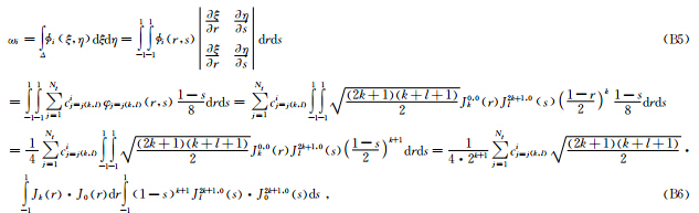
利用带参数的雅可比多项式的正交性:
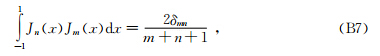

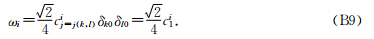
故,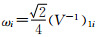
| [1] | Alford R M, Kelly K R, Boore D M. 1974. Accuracy of finite difference modeling of the acoustic wave equation[J]. Geophysics, 39(6): 834-842. |
| [2] | Barrett R, Berry M, Chan T F, et al. 1994. Templates for the Solution of Linear Systems: Building Blocks for Iterative Methods[M]. Philadelphia: SIAM. |
| [3] | Bos L, Taylor M A, Wingate M A. 2001. Tensor product Gauss-Lobatto points are Fekete points for the cube[J]. Mathematical of Computation-Math. Comput., 70(236): 1543-1547. |
| [4] | Briani M, Sommariva A, Vianello M. 2012. Computing Fekete and Lebesgue points: Simplex, square, disk[J]. Journal of Computational and Applied Mathematics, 236(9): 2477-2486. |
| [5] | Canuto C, Hussaini M Y, Quarteroni A, et al. 2007. Spectral Methods: Evolution to Complex Geometries and Applications to Fluid Dynamics. Scientific Computation[M]. Berlin and Heidelberg: Springer-Verlag, pp. 469. |
| [6] | Carcione J M, Wang P J. 1993. A Chebyshev collocation method for the wave equation in generalized coordinates[J]. Comp. Fluid. Dyn. J., 2: 269-290. |
| [7] | Chaljub E, Komatitsch D, Vilotte J P, et al. 2007. Spectral element analysis in seismology[J]. Advances in Wave Propagation in Heterogenous Earth, 48: 365-419. |
| [8] | Chen Q, Babuka I. 1995. Approximate optimal points for polynomial interpolation of real functions in an interval and in a triangle[J]. Comput. Methods Appl. Mech. Engrg., 128(3-4): 405-417. |
| [9] | Chen Q, Babuka I. 1996. The optimal symmetrical points for polynomial interpolation of real functions in the tetrahedron[J]. Comput. Methods Appl. Mech. Engrg., 137(1): 89-94. |
| [10] | Chew W C, Liu Q H. 1996. Perfectly matched layers for elastodynamics: A new absorbing boundary condition[J]. Journal of Computational Acoustics, 4(4): 341-359. |
| [11] | Collino F, Tsogka C. 2001. Application of the perfectly matched absorbing layer model to the linear elastodynamic problem in anisotropic heterogeneous media[J]. Geophysics, 66(1): 294-307. |
| [12] | de Basabe J D, Sen M K. 2010. Stability of the high-order finite elements for acoustic or elastic wave propagation with high-order time stepping[J]. Geophys. J. Int., 181(1): 577-590. |
| [13] | Dormy E, Tarantola A. 1995. Numerical simulation of elastic wave propagation using a finite volume method[J]. Journal of Geophysical Research, 100(B2): 2123-2133. |
| [14] | Dubiner M. 1993. Spectral methods on triangles and other domains[J]. J. Sci. Comp., 6(4): 345-390. |
| [15] | Faccioli E, Maggio F, Paolucci R, et al. 1997. 2D and 3D elastic wave propagation by a pseudo-spectral domain decomposition method[J]. J. Seism., 1(3): 237-251. |
| [16] | Fornberg B. 1988. The pseudospectral method: accurate representation of interfaces in elastic wave calculations[J]. Geophysics, 53(5): 625-637. |
| [17] | Graves R W. 1996. Simulating seismic wave propagation in 3D elastic media using staggered-grid finite difference[J]. Bul. Seism. Soc. Am., 86(4): 1091-1106. |
| [18] | Hesthaven J S. 1998. From electrostatics to almost optimal nodal sets for polynomial interpolation in a simplex[J]. SIAM J. Numer. Anal., 35(2): 655-676. |
| [19] | Hesthaven J S, Teng C H. 2000. Stable spectral methods on tetrahedral elements[J]. SIAM J. Sci. Comput., 21(6): 2352-2380. |
| [20] | Horn R A, Johnson C R. 1985. Matrix Analysis[M]. Cambridge: Cambridge University Press. |
| [21] | Kane C, Marsden J E, Ortiz M, et al. 1999. Variational Integrators and the Newmark Algorithm for Conservative and Dissipative Mechanical Systems [Ph. D. Thesis]. California: California Institute of Technology. |
| [22] | Karniadakis G E, Sherwin S J. 1999. Spectral hp Element Methods for CFD[M]. London: Oxford University Press. |
| [23] | Kelley C T. 1995. Iterative Methods for Linear and Nonlinear Equations[M]. Raleigh: North Carolina State University. |
| [24] | Kelly K R, Ward R W, Treitel S, et al. 1976. Synthetic seismograms: a finite difference approach[J]. Geophysics, 47(1): 2-27. |
| [25] | Khun M J. 1985. A numerical study of Lamb’s problem[J]. Geophys. Prosp., 33(8): 1103-1137. |
| [26] | Komatitsch D, Coutel F, Mora P. 1996. Tensorial formulation of wave equation for modeling curved interfaces[J]. Geophys. J. Int., 127(1): 156-168. |
| [27] | Komatitsch D, Vilotte J P. 1998. The spectral-element method: an efficient tool to simulate the seismic response of 2-D and 3-D geological structures[J]. Bull. Seism. Soc. Am., 88(2): 368-392. |
| [28] | Komatitsch D, Tromp J. 1999. Introduction to the spectral-element method for 3-D seismic wave propagation[J]. Geophys. J. Int., 139(3): 806-822. |
| [29] | Komatitsch D, Martin R, Tromp J, et al. 2001. Wave propagation in 2-D elastic media using a spectral element method with triangles and quadrangles[J]. Comput. Acoust., 9(2): 703-718. |
| [30] | Komatitsch D, Tromp J. 2002b. Spectral-element simulations of global seismic wave propagation-II. 3-D models, oceans, rotation, and self-gravitation[J]. Geophys. J. Int., 150(1): 303-318. |
| [31] | Komatitsch D, Tromp J. 2002a. Spectral-element simulations of global seismic wave propagation-I. Validation[J]. Geophys. J. Int., 149(2): 390-412. |
| [32] | Komatitsch D, Tromp J. 2003. A perfectly matched layer absorbing boundary condition for the second-order seismic wave equation[J]. Geophys. J. Int., 154(1): 146-153. |
| [33] | Krysl P, Endres L. 2004. Explicit Newmark/Verlet algorithm for time integration of the rotational dynamics of rigid bodies [Ph. D. Thesis]. California: University of California. |
| [34] | Lan H Q, Liu J, Bai Z M. 2011. Wave-field simulation in VTI media with irregular free surface[J]. Chinese J. Geophys. (in Chinese), 54(8): 2072-2084. |
| [35] | Lan H Q, Zhang Z J. 2011. Three-dimensional wave-field simulation in heterogeneous transversely isotropic medium with irregular free surface[J]. Bull. Seism. Soc. Am., 101(3): 1354-1370. |
| [36] | Lan H Q, Zhang Z J. 2012. Seismic wavefield modeling in media with fluid-filled fractures and surface topography[J]. Applied Geophysics, 9(3): 301-312. |
| [37] | Liu S L, Liu Y S, Wang W S, et al. 2013. Optimal generalized Shannon singular kernel convolution differentiator in seismic wavefield modeling[J]. OGP (in Chinese), 48(3): 410-416. |
| [38] | Liu Y S, Liu S L, Zhang M G, et al. 2012. An improved perfectly matched layer absorbing boundary condition for second order elastic wave equation[J]. Progress in Geophys. (in Chinese), 27(5): 2113-2122. |
| [39] | Liu Y S, Teng J W, Liu S L, et al. 2013. Explicit Finite Element Method with Triangle Meshes Stored by Sparse Format and its Perfectly Matched Layers Absorbing Boundary Condition[J]. Chinese J. Geophys.(in Chinese), 56(9): 3085-3099. |
| [40] | Lysmer J, Drake L. 1972. A Finite Element Method for Seismology[M]. Methods in Computational Physics. Academic: Academic Press. |
| [41] | Marfurt K J. 1984. Accuracy of finite-difference and finite-element modeling of the scalar and elastic wave equations[J]. Geophysics, 49(5): 533-549. |
| [42] | Martin R, Komatitsch D, Gedney S D. 2008. A variational formulation of a stabilized unsplit convolutional perfectly matched layer for the isotropic or anisotropic seismic wave equation[J]. CMES, 37(3): 274-304. |
| [43] | Mazzieri I, Rapetti F. 2012. Dispersion analysis of triangle-based spectral element methods for elastic wave propagation[J]. Numerical Algorithms, 60(4): 631-650. |
| [44] | Newmark N M. 1959. A method of computation for structural dynamics[J]. ASCE Journal of the Engineering Mechanics Division, 85(3): 67-94. |
| [45] | Padovani E, Priolo E, Seriani G. 1994. Low- and high-order finite element method: experience in seismic modeling[J]. J. Comp. Acoust., 86(2): 371-422. |
| [46] | Paolucci R, Faccioli E, Maggio F. 1999. 3D response analysis of an instrumented hill at Matsuzaki, Japan, by a spectral method[J]. J. Seism., 3(2): 191-209. |
| [47] | Pasquetti R, Rapetti F. 2004. Spectral element methods on triangles and quadrilaterals: comparisons and applications[J]. Journal of Computational Physics, 198(1): 349-362. |
| [48] | Pasquetti R, Rapetti F. 2006. Spectral Element Methods on Unstructured Meshes: Comparisons and Recent Advances[J]. Journal of Scientific Computing, 27(1-3): 377-387. |
| [49] | Pasquetti R, Rapetti F. 2010. Spectral element methods on unstructured meshes: which interpolation points?[J]. Numer. Algor., 55(2-3): 349-366. |
| [50] | Peter S. 1989. CGS: A fast Lanczos-type solver for nonsymmetric linear systems[J]. SIAM J. Sci. Stat. Comput., 10(1): 36-52. |
| [51] | Priolo E, Carcione J M, Seriani G. 1994. Numerical simulation of interface waves by high-order spectral modeling techniques[J]. J. Acoust. Soc. Am., 92(4): 681-693. |
| [52] | Richter G R. 1994. An explicit finite element method for the wave equation[J]. Appl Num. Math., 16(1): 65-80. |
| [53] | Saad Y. 2000. Iterative methods for sparse Linear systems[M]. 2nd ed, Philadelphia: SIAM,. |
| [54] | Sarma G S, Mallick K, Gadhingajkar V R. 1999. Nonreflecting boundary condition in finite-element formulation for an elastic wave equations[J]. Geophysics, 63(3): 1006-1016. |
| [55] | Seriani G, Priolo E, Carcione J M, et al. 1992. High-order spectral element method for elastic wave modeling[C]. // Expanded abstracts of the SEG, 62nd Int. Mtng of the SEG, New-Orleans, 1285-1288. |
| [56] | Sherwin S J, Karniadakis G E. 1995. A triangular spectrial element method: Applications to the incompressible Navier-stokes equations[J]. Comput. Methods Appl. Mech. Engrg., 123(1-4): 189-229. |
| [57] | Smith W D. 1975. The application of finite element analysis to body wave propagation problems[J]. Geophysical Journal of the Royal Astronomical Society, 42(2): 747-768. |
| [58] | Smith W D. 1980. Free oscillations of a laterally heterogeneous earth: A finite element approach to realistic modeling[J]. Physics of the Earth and Planetary Interiors, 21(2-3): 75-82. |
| [59] | Taylor M A, Wingate B A. 1998. Fekete collocation points for triangular spectral elements[J]. J. Num. Anal., 1-13. |
| [60] | Taylor M A, Wingate B A, Bos L P. 2007. A cardinal function algorithm for computing multiVariate Quadrature points[J]. Siam J. Num. Anal., 45(1): 193-205. |
| [61] | Tessmer E, Kosloff D. 1994. 3-D elastic modeling with surface topography by Chebyshev spectral method[J]. Geophysics, 59(3): 464-473. |
| [62] | Tromp J, Komatitsch D, Liu Q Y. 2008. Spectral-element and adjoint methods in seismology[J]. Communications in Computational Physics, 3(1): 1-32. |
| [63] | Virieux J. 1986. P-SV wave propagation in heterogeneous media velocity-stress finite-difference method[J]. Geophysics, 51(4): 889-901. |
| [64] | Virieux J. 1984. SH-wave propagation in heterogeneous media: velocity-stress finite-difference method[J]. Geophysics, 49(11): 1933-1942. |
| [65] | Wang T K, Fu X S, Zhu D X, et al. 2008. Spectral-element method for prestack reverse-time migration[J]. Progress in Geophysics (in Chinese), 23(3): 681-685. |
| [66] | Wang W S, Li X F, Lu M W, et al. 2012. Structure-preserving modeling for seismic wavefields based upon a multisymplectic spectral element method[J]. Chinese J. Geophys. (in Chinese), 55(10): 3427-3439. |
| [67] | Wang X M, Seriani G, Lin W J. 2007. Some theoretical aspects of elastic wave modeling with a recently developed spectral element method[J]. Science in China G: Physics, 50(2): 185-207. |
| [68] | West M, Kane C, Marsden J E, et al. 1999. Variational Integrators, the Newmark Scheme, and Dissipative systems[M]. Berlin: International Conference on Differential Equations. |
| [69] | Wingate B A, Boyd J P. 1996. Spectral element methods on triangles for geophysical fluid dynamics problems[A]. // Proc. Third International Conference on Spectral and High-order Methods, 305-314. |
| [70] | Zhang J F, Verschuur D J. 2002. Elastic wave propagation in heterogeneous anisotropic media using the lumped finite-element method[J]. Geophysics, 67(5): 625-638. |
| [71] | 兰海强, 刘佳, 白志明. 2011. VTI介质起伏地表地震波场模拟[J]. 地球物理学报, 54(8): 2072-2084. |
| [72] | 刘少林, 刘有山, 汪文帅,等. 2013. 最优化广义离散Shannon奇异核褶积微分算子地震波场模拟[J]. 石油地球物理勘探, 48(3): 410-416. |
| [73] | 刘有山, 刘少林, 张美根,等. 2012. 一种改进的二阶弹性波动方程的最佳匹配层吸收边界条件[J]. 地球物理学进展, 27(5): 2113-2122. |
| [74] | 刘有山, 滕吉文, 刘少林,等. 2013. 稀疏存储的显式有限元三角网格地震波数值模拟及其PML吸收边界条件[J]. 地球物理学报, 56(9): 3085-3099. |
| [75] | 王童奎, 付兴深, 朱德献,等. 2008. 谱元法叠前逆时偏移研究[J]. 地球物理学进展, 23(3): 681-685. |
| [76] | 汪文帅, 李小凡, 鲁明文,等. 2012. 基于多辛结构谱元法的保结构地震波场模拟[J]. 地球物理学报, 55(10): 3427-3439. |
| [77] | 王秀明, Seriani G, 林伟军. 2007. 利用谱元法计算弹性波场的若干个理论问题[J]. 中国科学, 37(1): 41-59. |