0 引言

地震波走时广泛应用于地震数据处理中，如叠前偏移(Zhao et al., 1998；Popovici and Sethian, 2002；刘国峰等，2009)、地震层析成像(Rawlinson and Kennett, 2008；张风雪等，2011；Liang et al., 2016；张明辉等，2019)及地震定位(Nelson and Vidale, 1990；Bai and Greenhalgh, 2006；De Kool and Kennett, 2014；赵爱华等，2015)等.走时计算的方法可以主要分为两大类：即射线追踪类方法(Zhang and Toksöz，1998；Zhao et al., 1992；Bai and Greenhalgh, 2005；Zhang and Thurber, 2005；Bai et al., 2010；Xu et al., 2006)和程函方程求解类方法(Vidale，1988；Podvin and Lecomte, 1991；Sethian and Popovici, 1999；Rawlinson and Sambridge, 2004b；Zhao，2005；Qian et al., 2007；孙章庆等, 2009, 2012；Waheed et al., 2015).射线追踪类方法的原理是沿程函方程的特征方向求解走时，这种方法在复杂速度模型中会出现焦散面和阴影区等问题(Xu et al., 2014, 2010).程函方程求解类方法有效避免了射线类方法的不足，且在计算精度和效率方面具有显著优势(Vidale, 1988, 1990；Rawlinson and Sambridge, 2004b)，因此，自提出以来发展迅速，逐渐成为走时计算的主流方法.

然而，起伏地表的处理一直是程函方程类方法的难点所在，需要在满足地震波传播的物理规律前提下，对起伏地形带来的不规则边界做灵活、稳定的处理，从而保证数值计算的精度和效率(侯爵等，2014).传统的程函方程类方法采用模型扩展的策略处理起伏地表(Hole，1992；Taillandier et al., 2009；Huang and Bellefleur, 2012；李勇德等，2016)，其核心思想是将起伏地形当作介质内部不连续面，通过填充低速介质将物理空间地形起伏的不规则模型扩展为计算空间的规则模型来处理.然而，该处理过程中采用的起伏地形的阶梯状表示及虚拟填充介质可能导致计算精度的损失(Ma and Zhang, 2015；郭高山等，2019).近年来逐渐提出的非结构化网格方法(Lelièvre et al., 2011；Bouteiller et al., 2018)可有效处理起伏地形，但其建模及走时求解算法颇为复杂、计算量大.Zhang and Chen(2006)在模拟起伏地表模型地震波场模拟时利用贴体网格构建的曲线坐标系方法巧妙地处理了地形起伏的难题，且兼有结构网格求解高效的优点.该方法自提出以来得到迅速发展(Lombard et al., 2007；Appelö and Petersson，2009；Lan and Zhang, 2011；Shragge，2016；Zhang et al., 2012, 2016；Sun et al., 2018). Lan和Zhang(2013a)将该处理方案引入至走时计算领域，为起伏地表下的的走时计算提供了一条新的途径.他们基于贴体网格的建模方式，推导建立了曲线坐标系的程函方程，该方程能够精确无损的刻画复杂地质模型的形态，并可用基于结构化网格的高效数值方法求解.同时，他们也针对性地发展了曲线坐标系程函方程的求解方法，包括Lax-Friedrichs扫描法(刘一峰和兰海强，2012；Lan and Zhang, 2013a，2013b)和迎风扫描法(Lan and Chen, 2018；Lan et al., 2018).然而，上述两种方法都存在震源奇异性问题(Vidale，1988；Fomel et al., 2009；Luo and Qian, 2011；Waheed and Alkhalifah, 2017)，如图 1所示，由于使用了平面波近似球面波，C点的数值解与真实解之间存在较大误差，且该误差随着迭代过程传播到整个计算空间.

震源奇异性的问题一直伴随程函方程的发展，多位学者就该问题进行过深入研究，主要解决方法包括源点网格加密(Rawlinson and Sambridge, 2004a；De Kool et al., 2006)，球坐标系程函方程(Alkhalifah and Fomel, 2010)以及因式分解(Fomel et al., 2009；Luo and Qian, 2011，2012；Noble et al., 2014；Treister and Haber, 2016).源点网格加密方法通过细化震源处网格，来减小源点处的截断误差，从而提高计算精度，但这种处理方式导致计算量增加，降低了算法的效率(Rawlinson et al., 2006).球坐标系程函方程的方法通过模拟球面波的传播来降低震源点误差，这种方法算法复杂，实际处理中难以有效应用.近年来，因式分解法受到越来越多的关注，该方法在没有明显增加计算量的情况下可从根源上解决震源奇异性的问题，且在各向同性和各向异性介质中都可应用.

针对曲线坐标系程函方程存在的震源奇异性问题，本文首先借鉴因式分解的思想，推导建立了曲线坐标系因式分解程函方程.然后，结合快速扫描法，发展了求解因式分解曲线坐标系程函方程的数值算法，从根源上解决了起伏地表的走时计算的震源奇异性问题.最后，通过数值实例，并与前人的方法进行详细的对比，全面分析测试新方法的优劣.

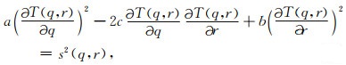
1 方法原理

曲线坐标系中，各向同性介质的程函方程可表示为

(1)

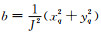
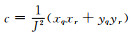
上述方程可以由笛卡尔坐标系(x, y)中的程函方程变换到曲线坐标系(q, r)得到(详见Lan and Zhang, 2013b).方程中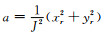，，这些参数刻画了起伏地形的局部特征，上述方程被称之为曲线坐标系程函方程.该方程可以描述任意地形起伏模型中地震波传播的走时规律.这里x_q表示，x_r，y_q，y_r，意义类似.J表示坐标变换的雅克比矩阵，J=x_qy_r-x_ry_q.当地形水平时，x_r，y_q退化为0，x_q，y_r退化为1.此时，雅克比矩阵J=1，方程(1)则退化为经典的程函方程.

为了解决震源奇异性问题，本研究对方程(1)进行因式分解.

首先，分别将走时T和慢度s分解成两个乘法因子：

(2a)

(2b)

其中T₀为已知因子，τ为未知因子，s₀为震源处的慢度，α为修正因子.这里T₀是以球面形式传播的，τ是在T₀附近的扰动，所以该方法很好地以球面波近似波前，规避了震源奇异性的问题.

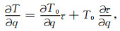
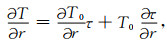
根据链式法则，走时偏导数表示如下：

(3a)

(3b)

将(3)式代入到方程(1)中，可以得到因式分解的曲线坐标系程函方程：

(4)

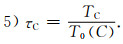
其中因子T₀可以解析求解，通过数值求解因子τ，可以精确计算走时值T，规避震源奇异性的问题，从而提高走时值T的精度.

本研究选择T₀为下列曲线坐标系程函方程的解：

(5)

其中(q₀, r₀)表示震源点的位置，此时a₀=a(q₀, r₀)，b₀=b(q₀, r₀)，c₀=c(q₀, r₀).

求解方程(5)，可得：

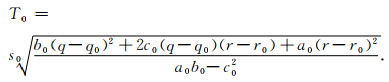
(6)

2 数值求解算法

本研究通过引入数学上用于求解静态Hamilton-Jacobi方程的方法(Luo and Qian, 2012)，用于求解曲线坐标系因式分解程函方程(4).该方法的关键在于局部解，即如何从一个点的周围网格点来求得可能的走时值.如图 2所示，在间距为h的矩形网格内部，待求的是C点的τ值，将方程(4)分别在相应的四个三角形上离散.例如，在三角形ΔCWS中，W=(x_W, y_W)，C=(x_C, y_C)，S=(x_S, y_S)，分别使用一阶差分近似τ的偏导数：

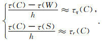
(7a)

将上式(7)代入方程(4)中，可以得到如下方程：

(7b)

关于τ(C)的一元二次方程(7b)，该方程的解有以下三种情况：①只有一个解；②有两个不同的解；③没有解.

如果①和②发生，需要判断得到的解是否满足如下的因果条件：通过C的特征向量T，

(7c)

在三角形的两边WC和SC之间，如图 2所示.

如果③发生时，利用特征线的方法，令特征向量T沿着三角形两边WC和SC.

例如，当特征向量T沿着WC时，则走时的侯选值为

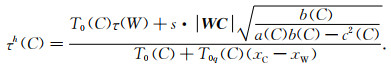
(7d)

然而，对于每一个三角形，τ(C)可能有多个满足因果条件的解，四个三角形中，则有更多可能满足因果条件的解，此时，需要从中选择令T值最小的τ(C)值作为当前τ(C)值的更新值.

基于上述局部算法，结合Gauss-Seidel扫描更新的全部策略，构建完整的快速扫描算法，具体如下：

1.初始化：在震源点上的τ值赋初值为1，即τ(q₀, r₀)=1.其他网格点上的τ初值设为一个较大的值(远大于所有计算点最终能算出的τ值)，这些点上的τ值在后续计算时会被更新.

2.Gauss-Seidel迭代：在交替的4个方向上，使用Gauss-Seidel型迭代法求解离散的非线性方程组，分别按四个方向扫描：

(1) i=1:I, j=1:J；(2) i=1:I, j=J:1，

(3) i=I:1, j=1:J；(4) i=I:1, j=J:1.

1) 每一个网格点处，在4个三角形ΔCEN，ΔCNW，ΔCWS和ΔCSE上离散方程(7b)，并在每个三角形上分别求解离散后的方程.例如，在三角形ΔCWS上，求解方程(7b)有两个可能的根，τ_{C, 1}和τ_{C, 2}.

2) 如果有两个实根，τ_{C, 1}和τ_{C, 2}

*如果τ_{C, 1}和τ_{C, 2}都满足因果条件，则

*如果只有τ_{C, 1}满足因果条件，则T_WS=τ_{C, 1}T₀(C)；

*如果只有τ_{C, 2}满足因果条件，则T_WS=τ_{C, 2}T₀(C)；

*如果τ_{C, 1}和τ_{C, 2}均不满足因果条件，用特征线方法沿着WC，SC得到τ_WC和τ_SC，并判断是否满足因果条件τ_WCT₀(C)≥T_W，τ_SCT₀(C)≥T_S，此时需要选择T_WS=min{τ_WCT₀(C), τ_SCT₀(C)}.

3) 如果方程(7b)没有实根，用特征线方法沿着WC，SC得到τ_WC和τ_SC，并判断是否满足因果条件τ_WCT₀(C)≥T_W，τ_SCT₀(C)≥T_S，此时需要选择T_WS=min τ_WCT₀(C), τ_SCT₀(C).

4) 从4个三角形中选择最小值，T_C=min{T_EN, T_NW, T_WS, T_SE}.

3.收敛判断：如果，那么迭代收敛并结束，δ是给定的收敛阈值.

3 计算实例

本研究通过3组数值实例测试了新方法计算地震波走时的精度和效率.模型1为水平地表模型，模型2为起伏地表模型，这两组模型中速度均设置为2 km·s^-1的均匀介质，将因式分解法与震源网格加密、迎风扫描法进行对比，并测试了不同的震源位置对结果的影响.模型3为相同的复杂地表模型，速度模型为Marmousi模型，测试新方法对复杂速度结构的适用性.

模型1：水平地表均匀介质

模型大小为1 km×1 km，均匀介质速度为2 km·s^-1，震源位于模型中心，模型表面水平.用四种不同精度的网格100×100，200×200，400×400，800×800分别离散该模型.本文将迎风扫描法、震源网格加密方法(如图 3所示)、因式分解法计算的走时结果与解析解的结果进行对比.由于篇幅限制，这里只展示网格精度为100×100的走时计算与对比结果(图 4).通过图 4可以看到，不同的方法都能够较好的吻合解析解，验证了本文方法的正确性，震源网格加密一定程度上能够降低震源奇异性的影响，但是，因式分解法表现出更高的计算精度.图 6进一步给出了这三种方法计算走时的绝对误差图，可以得出因式分解法具有更好的计算精度.

表 1对比了因式分解法与迎风扫描法两种方法不同网格精度下的L₁误差、迭代次数以及CPU时间.因式分解法计算走时的L₁误差比迎风扫描法计算走时的L₁误差明显较小，相差4~6个数量级.从迭代次数和CPU时间来看，两者的迭代次数都不随着网格精度的增加而增加，这对于高精度的走时计算至关重要.同时，因式分解法的迭代次数、所用的CPU时间更少，效率更高.主要原因在于，因式分解法的求解过程同样遵守了走时从已知到未知传播的物理规律，保持了迎风格式的优势，算法结构更为简洁，因此计算效率相对于Legendre形式的迎风快速扫描法计算效率更高；因式分解的过程本质上是对走时场的球面近似，因此能够更好的模拟震源点附近的高曲率的波前面，提高走时的计算精度.

为了进一步对比迎风扫描法、震源网格加密和因式分解法三者的精度.本文选取了地表处的走时曲线作为参考，对比三种方法的数值解和解析解之间的相对误差.从图 5再次证明了因式分解法的数值解与解析解更吻合，精度更高.网格加密的方法虽能够一定程度的提高精度，但是相对因式分解，其提高幅度有限.

模型2：起伏地表均匀介质

为了进一步测试因式分解法计算起伏地表走时的优势，选取Lan等文章中采用的数值模型(Lan and Zhang, 2013a, b).模型大小1.6 km×1.32 km，震源位于模型中央，地表由两个山峰和三个山谷组成，地形起伏较大，幅度从1.1 km到1.32 km，如图 7所示.本文使用4种不同精度的网格160×120，320×240，640×480，1280×960分别离散该模型.由于篇幅限制，这里只展示网格精度为160×120的走时场(图 8).从图 8中可以看出，起伏地表情况下，因式分解法的计算精度高.从表格2可以看出，因式分解法计算走时的L₁误差比迎风扫描法计算走时的L₁误差小，迭代次数和CPU时间也更小，说明因式分解法计算走时的精度和效率更高.图 10给出了两种方法计算走时的绝对误差图，可以看出迎风扫描法计算走时在源点处的误差较大，并且源点处的误差随着迭代过程逐渐传播到整个计算域，导致计算误差较大.这种现象的发生，主要是因为波是以球形方式传播到整个波场中，越靠近源点位置，波形曲率越大，以平面波的形式近似波前误差越大.而因式分解法很好地以球面波近似波前，规避了震源奇异性的问题，相对误差较小.相比于迎风扫描法的走时计算误差在坐标轴方向误差小而在对角线方向误差大，因式分解法计算的走时误差在各个方向都很均匀.这主要是由于迎风扫描法计算走时忽略了对角线上节点的信息，如图 1所示，基于平面波假设的迎风扫描法在对角线上(C点)会产生较大的误差，而轴线上的走时(A，B两点)误差小(Hassouna and Farag, 2007；卢回忆等，2013).从图 9和10也可以看到，地表处的走时误差相对较大，并且地形起伏越大，误差越大，这是由于贴体网格在地表处各向异性更强导致的走时误差增大(兰海强等，2012).此外，进一步测试不同震源深度对因式分解法计算走时的影响，图 11给出了不同震源位置处因式分解法计算走时的数值解与解析解的对比走时等值线图，可以看出不同震源位置处，因式分解法计算走时的精度都很高.

模型3：起伏地表复杂速度模型

为了测试新方法对复杂地表条件下复杂速度结构的适用性，在水平地表Marmousi模型的基础上修改为起伏地表模型，同时对模型进行一定的高斯光滑，其速度结构如图 12所示.同样，使用不同网格精度分别离散该模型：160×120，320×240，640×480，1280×960.限于篇幅，这里只展示网格精度为160×120的走时计算与对比结果(图 13).图 14为地表处的数值解和解析解的对比图，图 15进一步给出了两种方法在全局域的数值解和解析解的对比图.可以看出，因式分解法相比于迎风扫描法精度更高，这里使用的高阶Lax格式作为真实解，结果显示，因式分解法与真实解吻合更好，验证了新方法对复杂速度模型的有效性.图 16给出了未进行光滑的Marmousi模型对应的误差图，同样可以看出，因式分解法相比于迎风扫描法，精度仍然较高，但提高较为有限.此外，从表 3中可以看出，因式分解法计算走时的L₁误差比迎风扫描法计算走时的L₁误差小，迭代次数和CPU时间都较小.该模型充分证明了因式分解法计算复杂地表和复杂速度模型的走时方面具有显著的优势.

4 结论与讨论

本文借鉴因式分解的思想，推导建立了因式分解的曲线坐标系程函方程，并结合快速扫描法，发展了相应的数值求解算法，极大地降低了走时计算的误差，从而提高算法的精度.通过数值模型，将因式分解法与迎风扫描方法、震源网格加密方法做了详细对比(计算精度和效率).论证了因式分解法求解曲线坐标系程函方程的优越性.结果表明：

(1) 因式分解的曲线坐标系程函方程有效规避了震源奇异性问题，提高了震源处走时的计算精度，从而显著提高整个模型空间的求解精度.

(2) 相较于迎风扫描法，因式分解法的震源计算精度明显提高，且计算效率不会随着网格精度增加而降低.

然而，因式分解法在处理强速度间断面时对精度的提高较为有限，这可能是由于因式分解基于的扰动理论在强速度间断面情况下效果不够显著，有待进一步研究.

目前，本文中的因式分解法只应用到求解二维曲线坐标系程函方程.但随着三维地震勘探的广泛应用，对三维复杂地表模型的走时计算精度提出了更高的要求.下一步拟将因式分解快速扫描法拓展到三维曲线坐标系程函方程的计算，为三维复杂地表条件下地震走时数据的高精度成像提供方法基础.

致谢  感谢美国爱荷华州立大学的Songting Luo博士提供程序和建设性意见.感谢英国剑桥大学Rawlinson Nicholas教授提供2D-FMM程序.特别感谢两位评审专家为本文完善提出的宝贵意见.