 2020, Vol. 63


2. 中国地质大学(北京)地球物理与信息技术学院, 北京 100083;
3. 防灾科技学院地球科学学院, 河北三河, 065201
2. School of Geophysics and Information Technology, China University of Geosciences, Beijing 100083, China;
3. School of Earth Sciences, Institute Disaster of Prevention Science and Technology, Hebei Sanhe 065201, China
联合反演是指同时反演多种地球物理数据,利用不同物性参数,从不同角度反映地质构造属性,通过岩石物性关系或者结构耦合关系约束不同物性参数的分布,得到合理的地质-地球物理模型,即所获得的地质-地球物理模型能同时拟合多种地球物理数据.地球物理联合反演方法可以有效结合不同地球物理方法的优势,减小反演多解性,提高反演精度(Vozoff and Jupp, 1975; 高锐, 1995; 杨辉等, 2002; 敬荣中等, 2003; 吕庆田等, 2015).
基于岩石物性关系的联合反演方法,可很好地促进岩石物性耦合,在解决复杂地质构造方面得到了成功应用(Dobróka et al., 1991; 杨振武等, 1998; Arie et al., 1997; Colombo and De Stefano, 2007; 于鹏等, 2009; 陈晓等, 2010, 2016).但该方法在实际应用中对先验信息依赖性比较强,具有局限性.Gallardo和Meju于2003、2004年根据反映地质体的不同物性参数之间存在相似边界的假设,提出了交叉梯度结构耦合法.该方法不依靠岩石物性关系,提供了一种简单而且广义的评价模型结构相似度的标准,适用于不同地球物理方法的联合反演,为联合反演带来了新思路.国内外学者利用这一方法进行了各种地球物理数据联合反演研究,取得了大量研究成果(Gallardo and Meju, 2003, 2004; Gallardo, 2007a; Linde et al., 2006; Hu et al., 2009; Moorkamp et al., 2011a; Abubakar et al., 2012; Um et al., 2014; 彭淼等, 2013; Molodtsov et al., 2013; Bennington et al., 2015; 李桐林等,2015; 李兆祥等, 2015; Peng et al., 2019; 张镕哲等, 2019; Wu et al., 2020).
电阻率法是电法勘探的经典分支方法,从电性角度揭示地下介质的非均匀性特征,在金属矿、水文、工程、环境等领域得到了广泛应用(Yuval and Oldenburg, 1996; 吴小平和徐果明, 2000; 吴小平和汪彤彤, 2001; Hauck, 2002; Krautblatter and Hauck, 2007; 汤井田等, 2007; Jones and Pascoe, 1971; Barde-Cabusson et al., 2013; 李术才等, 2015).电阻率法通过改变供电极距的大小控制勘探深度,通过采用大极距供电,可对深达上千米的地下目标体进行有效探测.
背景噪声法(Weaver, 2005; Roux et al., 2005; Shapiro et al., 2005; Yao et al., 2006, 2008; Li et al., 2009)以自然现象产生的低频微动或人类活动产生的高频微动作为信号源,因该方法对环境无破坏、施工便捷、经济效益高等优势,被广泛应用于城市物探、资源探测、深部结构探测等领域.背景噪声法通过选择频段来控制探测深度,长周期面波数据可用以研究地壳深部结构,高频面波数据可用以研究浅层几百米的速度结构信息.
对于电阻率法和背景噪声法,通过选择供电极距大小和面波频段,确定两种方法共同的有效探测深度,发挥两种方法对地下介质电阻率和速度参数反映能力的优势,通过联合反演技术实现优势互补,可以减少反演多解性,提高反演精度.
实现电阻率法和背景噪声法的三维联合反演首先需要构建电阻率和速度参数的耦合关系.已有研究表明在局部熔融\半熔融异常体、含水的裂隙或断层、壳内滑脱层等特殊构造区,速度模型和电阻率模型在三维结构分布上具有相似性(Newman et al., 2008; Berdichevsky and Dmitriev, 2008),已有研究学者利用这一特性实现了电阻率法和地震体波走时联合反演(Infante et al., 2010; 高级和张海江, 2016; 高级等, , 2017; Shi et al., 2017; Demirci et al., 2017).由于传统面波频散“两步”反演法具有局限性,目前还没有见到电阻率法和背景噪声法的三维联合反演研究成果.背景噪声法不受地震发生方位和发震时刻的约束,对地下剪切波速度反映灵敏,相比体波走时法具有优越性.
基于速度和电阻率结构耦合的联合反演,可以实现优势互补,相互验证,提高反演结果的可靠性和一致性,具有实用价值.本文采用Fang等(2015)提出的面波频散数据直接反演三维剪切波速度结构的思路,开展了背景噪声法和电阻率法三维联合反演研究工作.采用有限内存拟牛顿法(L-BFGS)实现了电阻率法和背景噪声法单方法三维反演;基于速度和电阻率的结构耦合约束,实现了电阻率法和背景噪声法的三维联合反演研究;通过复杂模型合成数据算例检验了算法的稳定性和可靠性,对比单方法反演结果,展示了联合反演算法的优越性.
1 电阻率法和背景噪声法三维联合反演理论 1.1 交叉梯度函数交叉梯度函数(Gallardo and Meju, 2003, 2004)通过定义两种不同物性参数的梯度的叉乘来定量描述两种物性参数的结构相似性,是实现两种物性参数模型之间相互约束的关键,适用于不同地球物理方法联合反演研究.
根据定义可将电阻率和速度模型的交叉梯度函数表达式写成:

|
(1) |
mr表示电阻率模型,ms表示速度模型.
联合反演中的交叉梯度项为t三分量的平方和,可以写成:
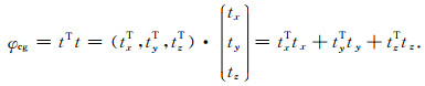
|
(2) |
将t对m(m代表mr或ms)在m0处进行泰勒级数展开,忽略一阶以上的偏导数项,可得
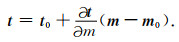
|
(3) |
当反演的初始模型为均匀半空间时t0=0.根据闫政文等(2020)的公式推导,将


|
(4) |
不同的学者从不同的角度出发,针对如何实现交叉梯度约束的联合反演提出了不同的策略,主要有:在满足单方法目标函数的同时要求交叉梯度函数(公式1)等于零(Gallardo and Meju, 2003, 2004);将单方法反演的结果通过交叉梯度函数修正后的模型作为初始模型继续迭代(Um et al., 2014; 高级等, 2017);将交叉梯度项加入单方法目标函数中构建两个联合反演目标函数(Hu et al., 2009; 彭淼等, 2013).本文采用Hu等(2009)和彭淼等(2013)提出的构建两个联合反演目标函数的策略,在两个联合反演目标函数中,引入结构耦合约束项,采用交替迭代法交替更新速度和电阻率模型.该方法属于弱耦合约束,在保证单方法反演拟合数据的前提下,寻找速度和电阻率模型结构更为相似的模型.具体公式推导和反演流程如下.
将交叉梯度项(式(2))分别通过权重因子加入到背景噪声法和电阻率法的单方法反演目标函数中,形成两个联合反演目标函数,具体表示如下:
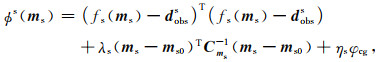
|
(5) |
|
(6) |
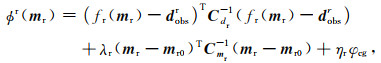
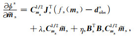
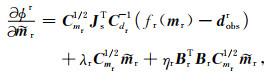
ϕs(ms)为背景噪声法联合反演目标函数,ϕr(mr)为电阻率法联合反演目标函数,ms, mr分别为三维介质速度模型和电阻率模型,dobss, dobsr分别为背景噪声法和电阻率法实测数据,fs(·), fr(·)为背景噪声法和电阻率法正演算子Cdr-1为电阻率法的数据协方差矩阵的逆矩阵,Cms-1和Cmr-1为速度模型和电阻率模型协方差矩阵的逆矩阵,λs, λr为拉格朗日因子,ηs, ηr为交叉梯度项权重因子.
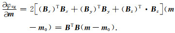
求解联合反演目标函数(式(5)、(6))对模型ms, mr的偏导数,可以写成:
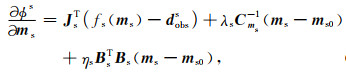
|
(7) |
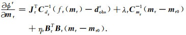
|
(8) |
Js和Jr分别表示背景噪声法和电阻率法数据的灵敏度矩阵.Br和Bs为公式4中对应B矩阵(即

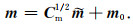
为了提高反演的稳定性,对模型m进行如下变换,对目标函数的梯度项进行光滑(Egbert and Kelbert, 2012):
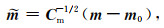
|
(9) |
则目标函数的梯度可以改写成:
|
(10) |
|
(11) |
采用L-BFGS迭代法求解联合反演目标函数及其梯度,采用双循环归隐式避免海森矩阵的存储(Byrd et al., 1994).在获取
|
(12) |
电阻率法三维正演采用一次场和二次场分解算法(马欢等,2018).通过解析法或数字滤波法求解一次电位(均匀半空间或层状介质模型产生的电位),采用有限差分法求解二次电位(剩余电阻率模型产生的电位).
背景噪声频散数据正演是基于一维水平层状介质模型计算地表每个网格的速度频散,通过FMM射线追踪法获取面波不同周期在地表的传播路径,然后求解面波不同周期沿着不同射线路径的走时,获得理论频散数据(Fang et al., 2015).
在求解联合反演目标函数的极小值时,采用交替迭代法,在满足单方法反演拟合差要求的情况下,寻找速度和电阻率模型结构更为相似的模型,具体流程见图 1,简要地可以概括为如下几个步骤:

|
图 1 电阻率法与背景噪声法三维联合反演流程图 Fig. 1 Flow chart of 3-D joint inversion of resistivity method and ambient noise method |
(1) 输入初始速度模型ms0和初始电阻率模型mr0;
(2) 分别进行电阻率法和背景噪声法单独反演,经过几次迭代,当反演的速度和电阻率有一定的异常形态之后,判断是否准备开始联合反演计算;
(3) 当判断可以开始联合反演时,将最新的速度和电阻率模型通过交叉梯度函数,计算交叉梯度项,代入联合反演公式(5)和(6),初始模型为最近一次迭代后的最新模型;
(4) 通过计算联合反演公式,得到带有结构耦合约束的速度和电阻率模型,然后判断是否更新交叉梯度项.如果不更新,则按照上次的交叉梯度项继续迭代计算.如果更新,则将最新的速度和电阻率模型重新计算交叉梯度函数,重新代入联合反演公式进行计算;
(5) 每次迭代更新模型的时候,都进行判断是否满足迭代终止条件,如果满足则终止迭代,如果不满足则继续迭代计算.
单方法和联合反演迭代的终止条件为数据拟合差趋近于/等于期望值或迭代次数达到设定值.联合反演的结果不仅满足单方法的迭代终止条件,还能满足交叉梯度值最小,寻求速度和电阻率结构更为一致的模型.
2 规则体组合模型三维联合反演试算 2.1 规则体组合模型设计和正演计算为了测试三维联合反演算法的有效性,本文通过多个规则体组合成一套具有实际地质意义的三维模型(图 2a),图中每个模型块体与实际构造体相似,其中E类似于基底构造,C类似于低速低阻地垒或者盆地构造,C构造体的四周与基底E是近垂直的接触带,B1和B2是在C构造中两个低速高阻异常体.B1和B2异常值一样,规模和埋深不一样.

|
图 2 三维规则体组合模型示意图及三维模型三个不同位置的模型切片图 (a)三维规则体组合模型示意图; (b)模型在Z=250 m深度处的水平切片图; (c)模型在Y=300 m处沿X方向的垂直剖面图; (d)模型在X=900 m处沿Y方向的垂直剖面图. Fig. 2 3-D model composed of regular anomalies and three slice diagrams of model (a) 3-D model composed of regular anomalies; (b) The horizontal slice diagram of model with Z=250 m; (c) The vertical slice diagram of model with Y=300 m; (d) The vertical slice diagram of model with X=900 m. |
从三个不同的切片图剖析三维模型特征.图 2b是三维模型在Z=250 m深度处的水平切片图,该切片图中包含有低速低阻体C和两个低速高阻体B1、B2.图 2c为模型在Y=300 m处沿X方向的垂直剖面图,构造体C与基底E是近垂直向内的接触构造,异常体B1和B2为位于构造体C内的两个规则体.图 2d为模型在X=900 m处沿Y方向的垂直剖面图,构造体C与基底E是近垂直向外的接触构造,异常体B2为独立的长方形异常.模型的具体物性参数分布见表 1(表中速度采用δv/v值,即为异常体与背景速度差除以背景速度,采用线性递增的背景速度模型).
|
|
表 1 规则体组合模型的速度和电阻率参数设计 Table 1 Velocity and resistivity parameters of 3-D model composed of regular anomalies |
电阻率法和背景噪声法正演对网格剖分的要求不一样.为了满足边界条件的要求,电阻率法正演的剖分区域比较大,同时考虑到分辨率随深度增加而降低的特点,一般采用不等间隔剖分.水平方向在目标研究区为等间隔剖分,研究区外水平网格间距逐渐增大(图 3a),垂直方向在目标深度范围内采用等间隔剖分,更深处的网格间距逐渐增大(图 3c).背景噪声法的网格剖分在水平方向采用等间距剖分(图 3b),在垂直方向因考虑到面波周期越长,垂向分辨率越低(Fang et al., 2015),所以在垂直方向目标研究区的深度范围采用等间隔剖分,更深处的网格间距逐渐增大(图 3d).联合反演中选取两种方法的中间有相同网格剖分区域(图 3中黑色方框)作为交叉梯度约束区,在约束区外围的网格上不进行交叉梯度约束.

|
图 3 电阻率法(a、c)与背景噪声法(b、d)水平和垂向网格剖分图 (a)和(b)为X-Y平面网格剖分;(c)和(d)为X-Z网格剖分图;黑色框为交叉梯度计算范围 Fig. 3 Model discretization showing the grid nodes used in the resistivity inversion (a, c) and the grid cell in the ambient noise inversion (b, d) (a) and (b) represent the grid nodes in X-Y; (c) and (d) represent the grid nodes in X-Z; the black rectangles show the common region for joint inversion. |
背景噪声法的测点观测设有16个虚源,间距为1600 m(图 4a,红色星号).接收点有64个(图 4a),间距为800 m(图 4a,蓝色三角形),周期为0.2~3 s的Rayleigh波群速度频散数据,用于反演的频散数据需要考虑孔径与周期的关系,本文选择每条射线路径至少包含2个波长(Li et al., 2009, 2019).图 4a为虚源位于(2300,2300)到三个接收点(-2900,-2900,红色)、(1100,-2900,蓝色)、(-2900,1100,黑色)不同周期的射线分布,图 4c为这三个台站对的理论频散曲线(Syn 1, 2, 3),图中可以看出穿过低速体B1和B2的面波频散路径频散曲线(红色标志),相比黑色和蓝色的射线路径的频散速度值要低,随着周期变大,三条频散曲线变化趋势趋于一致.图 4b为线性递增速度模型的0.2~1.5 s背景噪声频散数据核函数,从这几个周期的核函数特征可以看出本文选取的频段可以在地下1000 m范围为有较好的分辨率,尤其对500 m以内的灵敏程度更高.

|
图 4 背景噪声三个台站对的不同周期的射线路径(a),周期为0.2~1.5 s的面波核函数(b),频散曲线正演响应图(c) 图a中虚源位于(2300, 2300)到三个接收点(-2900,-2900,红色,标注1)、(1100,-2900,蓝色,标注2)、(-2900,1100,黑色,标注3)的每个周期的射线分布. Fig. 4 The ray paths of three station pairs with different period of surface wave (a), the depth kernel of surface wave from 0.2 s to 1.5 s (b), the forward dispersion curves (c). (a) The ray distribution from virtual source (2300, 2300) to three receiving sites (-2900, -2900, red line, marked 1), (1100, -2900, blue line, marked 2), (-2900, 1100, black line, marked 3). |
电阻率法的数据体是这样形成的:采用二极测深装置(A极供电,M极接收,B和N极位于无穷远),在目标研究区5 km×5 km范围内布设了25个供电点(图 5中红色带圈十字符号),每个供电点覆盖的测量范围为1.6 km×1.6 km(图 5中黑色方框),在1.6 km×1.6 km的测量范围内布设了64个测点(图 5b中黑色点).对于这样的数据体,电阻率法探测深度可达500 m以上,跟背景噪声法的探测深度相匹配.图 5b为供电点位于(-100, -100)的理论模型正演的视电阻率平面等值线图,由于点源位于低阻体C上,所以在离点源近的测点视电阻率值低,随着极距增加逐渐反映深部电阻率的信息.

|
图 5 电阻率法观测装置(a)及点源位于(-100, -100)模型正演视电阻率分布(b) 红色带圈十字为点源; 黑色点为接收点; 黑色方框分别为点源位于(-100, -100)的观测范围. Fig. 5 The observation geometry (a) of the resistivity method and the forward apparent resistivity (b) of the synthetic model of the source at (-100, -100) The red circle cross represent sources; the black dots represent receivers; the black boxes show the observation ranges of the sources located at (-100, -100) |
对上述的模型和观测装置正演的视电阻率值和频散数据,加入5%的高斯随机误差,形成电阻率法和背景噪声法的理论模型合成数据,作为测试单方法和联合反演的观测数据.背景噪声反演初始速度模型为线性递增模型,电阻率法反演初始电阻率为均匀半空间(100 Ωm)模型.
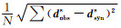
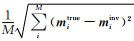
为了定量评估反演结果,分别定义和计算了电阻率法和背景噪声法单方法和联合反演结果的数据拟合差(RMS)、真实模型和反演模型差(RES)和交叉梯度函数值(|t|).
电阻率法RMS用公式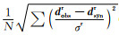
从图 6RMS曲线变化趋势可知ANT和DC单方法和联合反演都具有较好的收敛性.表 2为单方法(SP)和联合反演(JT)相应的RMS、RES、|t|统计结果.从表中,可以发现联合反演后的电阻率法的RMS值由1.355降到1.293、mean |RES|值由7.3901降到6.6867.背景噪声法的数据拟合差从1.7522×10⁻⁵降到1.3386×10⁻⁵、mean |RES|值由0.0297降到0.0255.单方法反演结果的交叉梯度值也由6.5×10⁻³降到2.2×10⁻³.总体上可以发现联合反演后的结果在RMS、RES和t值上优于单方法结果,这说明联合反演的结果不仅仅可以满足数据拟合差的要求,还可以获得速度和电阻率模型结构上更相似的结果.

|
图 6 规则体组合模型单方法和联合反演迭代RMS曲线图 (a)背景噪声法单方法和联合反演迭代RMS曲线图;(b)电阻率法单方法和联合反演迭代RMS曲线图.空心圈曲线为单方法反演迭代RMS曲线;实心点曲线为联合反演迭代RMS曲线. Fig. 6 Plots of RMS iteration curves for separate and cooperative inversion in the combined model with regular anomalies (a) Represents the plots of RMS iteration curves for separate and cooperative inversion of ANT method; (b) Represents the plots of RMS iteration curves for separate and cooperative inversion of DC method. The curves with hollow circles represent the RMS iteration of separate method; The curves with solid dots represent the RMS iteration of separate method. |
|
|
表 2 单方法和联合反演结果的RMS、RES和|t|值 Table 2 The values of RMS、RES and |t| derivated from separate and joint inverted models |
下面结合速度、电阻率模型的水平切片图和垂直剖面图分别对单独反演和联合反演结果进行分析.
图 7是单方法反演结果、联合反演结果和交叉梯度值在Z=250 m深度的水平切片图.根据图 2b可知,该切片图主要展示低速低阻体C和两个低速高阻体B1、B2.图 7(a1)和(a2)为背景噪声法单方法反演和联合反演的结果,可见两种反演的结果类似,可以把异常体C、B1和B2的边界和速度值恢复得跟真实值相近,但从反演细节来看,可以发现联合反演后的异常体B1速度值恢复得比单方法结果更好,在C与基底E的边界处的刻画更清晰;该切片的mean |RES|从单独反演的4.1602×10⁻²下降到联合反演的2.6842×10⁻²,表明联合反演的结果与真实模型更相近.

|
图 7 单方法反演和联合反演结果在Z=250 m深度处的水平切片图 (a1)、(b1)单方法反演获得的速度和电阻率模型; (a2)、(b2)联合反演获得的速度和电阻率模型;(a3)、(b3)单方法反演和联合反演结果的交叉梯度图. mean |RES|为对应水平切片的反演结果与模型差值;mean |t|为对应水平切片单方法和联合反演结果的交叉梯度值. Fig. 7 The horizontal section at Z=250 m calculated from the separate and the joint inversion of DC and ANT (a1) and (b1) represent the separately inverted velocity and resistivity models; (a2) and (b2) represent the jointly inverted velocity and resistivity models; (a3) and (b3) represent the cross-gradient values from separate and joint velocity and resistivity models. mean |RES| represent the model differences of the corresponding horizontal slice; mean |t| represent cross-gradient value of the corresponding horizontal slice. |
图 7(b1)和(b2)为电阻率法单方法反演和联合反演的结果,可见联合反演的结果相比电阻率法单方法反演结果在C、B1和B2的边界附近有明显的改善;mean |RES|从单方法反演的15.042下降到联合反演的12.0786.B1的埋深比B2深,单方法反演结果对B1和B2异常体都有反应,B2的电阻率值和异常形态恢复要比B1好.经过联合反演之后,异常体B1、B2、C和E之间的边界分辨率明显提升,B2的边界与真实边界更接近,B1的异常形态恢复得更好些,电阻率值相比单方法反演结果也有明显改善.图 7(a3)和(b3)为单方法反演和联合反演结果在此切片上的速度和电阻率交叉梯度图,可见在异常体边界附近联合反演结果对应的交叉梯度值明显减小.交叉梯度值mean |t|从单方法反演的1.818×10⁻²下降到联合反演的0.81675×10⁻²,表明联合反演获得的速度和电阻率结构更相似.
图 8的剖面图(图 2c)主要展示了异常体C与基底E的近垂直向内接触构造、埋深和规模不同的异常体B1和B2.(图 8a1)和(图 8a2)为背景噪声法单方法反演和联合反演结果,跟上述水平切片的结果一样,两种反演方法的结果相似,在C与E两侧近垂直向内的接触带及其底边界分界处、B1和B2边界和速度值都有很好的恢复.联合反演结果在异常体边界的刻画要比单方法反演结果有一定的改善,mean |RES|从单方法反演的5.2599×10⁻²下降到联合反演的4.6032×10⁻².

|
图 8 单方法反演和联合反演结果在Y=300 m处沿X方向的垂直剖面图 (a1)、(b1)单方法反演获得的速度和电阻率模型; (a2)、(b2)联合反演获得的速度和电阻率模型;(a3)、(b3)单方法反演和联合反演结果的交叉梯度图. Fig. 8 The slice section at Y=300 m calculated from the separate and joint inversion of the resistivity method and the ambient noise method (a1) and (b1) represent the separately inverted velocity and resistivity models; (a2) and (b2) represent the jointly inverted velocity and resistivity models; (a3) and (b3) represent the cross-gradient values from separate and joint velocity and resistivity models. |
图 8(b1)和(b2)为电阻率法单方法反演和联合反演结果.可见单方法反演对C和E之间近垂直的构造特征、B1和B2独立圈闭的异常体的反演效果不明显,在异常体B1处虽然能看出有异常,但完全分辨不出一个独立的异常体,可能被理解成隆起构造,B2虽然异常特征比B1明显,但是没有形成独立圈闭的异常体构造.联合反演对深部电阻率信息有明显的提升,异常体B1和B2底部与C的边界清晰,呈现出独立的、圈闭的异常体特征.C和E两边近垂直向内的接触带的分辨率有明显的提升,联合反演改善了深部电阻率的分辨率.联合反演获得的速度和电阻率的交叉梯度值相比单方法反演结果有明显的改善(图 8a3和b3),mean |t|从单方法反演的2.0961×10⁻²下降到联合反演的0.64774×10⁻²,在异常体B1和B2周边、C和E接触带的交叉梯度值明显减小.
图 9剖面图(图 2d)主要展示异常体C与基底E的近垂直向外接触构造、独立长方形的异常体B2.背景噪声法单方法反演和联合反演结果的特征与图 8类似,不再详细叙述.电阻率法单方法反演结果(b1)显示,异常体B2呈现拖尾的现象,与E相连通.联合反演结果(b2)显示,异常体B2的异常形状和电阻率值有明显的改善;异常体C与E的左右边界、下边界的分辨率明显提升;交叉梯度值(b3)在边界处明显降低.

|
图 9 单方法反演和联合反演结果在X=900 m处沿Y方向的垂直剖面图 (a1)、(b1)单方法反演获得的速度和电阻率模型; (a2)、(b2)联合反演获得的速度和电阻率模型;(a3)、(b3)单方法反演和联合反演结果的交叉梯度图. Fig. 9 The slice section at X=900 m calculated from the separate and joint inversion of the resistivity method and the ambient noise method (a1) and (b1) represent the separately inverted velocity and resistivity models; (a2) and (b2) represent the jointly inverted velocity and resistivity models; (a3) and (b3) represent the cross-gradient values from the separately and jointly inverted velocity and resistivity models. |
对比单方法反演和联合反演结果的不同块体的物性交会图(图 10),可以发现构造体C(红色点)中横向和纵向均相对单方法更加收敛于真实值附近,反演结果稳定.基底E(蓝色点)物性值也表现更加收敛集中于真实值附近,C和E之间存在线性过渡的趋势,这是因为C和E是相邻的两个块体,在反演过程中受到模型光滑(正则化项)作用的影响,所以反演结果会有线性过渡趋势.异常体B1和B2具有相同物性,但规模、埋深不一样,虽然单方法反演和联合反演结果都没有把B1和B2的物性值完全恢复到真实值附近,但从交会图的变化趋势依然能看出联合反演结果优于单方法反演结果.单方法反演中,B1和B2的反演结果交叉的混叠在一起,分不清有两种异常体的存在,经过联合反演之后,可以清晰的发现B1/B2与C异常体的过渡区有两条清晰的线性变化趋势,说明联合反演之后的结果通过交会图可以将B1、B2两个异常体分开,相比单方法反演结果具有优越性.

|
图 10 单方法反演结果(a)和联合反演结果(b)的物性交会图 红色点表示异常体C速度和电阻率交会点; 黄色点表示异常体B2速度和电阻率交会点; 绿色点表示异常体B1速度和电阻率交会点; 蓝色点表示基底E速度和电阻率交会点.C、E、B1/B2标注的坐标位置为模型真实物性值. Fig. 10 The cross-plots of resistivity and velocity models from the separate (a) and joint (b) inversion results The red dots represent the resistivity and velocity values obtained from anomaly C; the yellow dots represent the resistivity and velocity values obtained from anomaly B2; the green dots represent the resistivity and velocity values obtained from anomaly B1; the blue dots represent the resistivity and velocity values obtained from basement E. The coordinate positions marked with C, E and B1/B2 are the real physical property values of the model. |
为了进一步检验三维联合反演算法在实际不规则复杂地质模型的有效性,本文从实际三维物理模型中提取出不规则异常体的形状(图 11),并设置各个不规则体为恒定异常值.图中红色异常体为低速低阻异常体(δv/v为-0.2,ρ为10 Ωm),蓝色异常体为高速高阻异常(δv/v为0.2,ρ为400 Ωm).背景速度为随深度线性递增模型,背景电阻率值为100 Ωm.观测装置、正反演网格等参数与上述模型相同.图 11(b、c、d)分别为三维模型在Z=100 m水平切片、X=-300 m和Y=-100 m处的垂直剖面图.为了便于识别每个切片中的异常体,图中分别对各个异常块体进行标注(“L”表示低速低阻体,“H”表示高速高阻体,从1开始对每个切片中独立异常体进行编号).

|
图 11 三维不规则体组合模型示意图及三维模型在三个不同位置的模型切片图 (a)三维不规则体组合模型示意图; (b)模型在Z=100 m深度处的水平切片图; (c)模型在Y=-300 m处沿X方向的垂直剖面图; (d)模型在Y=-100 m处沿X方向的垂直剖面图. Fig. 11 The diagram of the 3D model composed of irregular anomalies and three slice diagrams of the model (a) The diagram of the 3-D model composed of irregular anomalies; (b) the horizontal slice diagram of model with Z=100 m; (c) The vertical slice diagram of model along X=-300 m; (d) The vertical slice diagram of model along Y=-100 m. |
基于本文开发的单方法和联合反演算法,对不规则体组合模型进行理论模型合成数据反演试算.图 12为ANT和DC单方法和联合反演迭代RMS曲线图,从RMS变化趋势可知ANT和DC单方法和联合反演都具有较好的收敛性,联合反演后的RMS相比单方法反演结果有所下降.背景噪声法的数据拟合差从9.452×10⁻⁶降到9.197×10⁻⁶,电阻率法的数据拟合差从6.563降到5.126.

|
图 12 不规则体组合模型单方法和联合反演迭代RMS曲线图 (a)背景噪声法单方法和联合反演迭代RMS曲线图; (b)电阻率法单方法和联合反演迭代RMS曲线图.空心圈曲线为单方法反演迭代RMS曲线; 实心点曲线为联合反演迭代RMS曲线. Fig. 12 Plots of RMS iteration curves for the separate and joint inversion in the 3-D model composed of irregular anomalies (a) Represents the plots of RMS iteration curves for the separate and joint inversion of the ANT method; (b) Represents the plots of RMS iteration curves for the separate and joint inversion of the DC method. The curves with circles represent the RMS iteration of the separate inversion method; the curves with dots represent the RMS iteration of the joint inversion method. |
图 13是单方法和联合反演结果在Z=100 m深度的水平切片图.图 13(a1)和(a2)为背景噪声法单方法和联合反演结果,图中可知两种反演结果在该切片的异常体特征相似,对低速异常体(L1~L5)和高速异常体(H1~H3)都可以恢复得跟真实模型差不多.从异常体的异常值来看,联合反演后的结果相比单方法反演结果更接近于真实模型值,mean |RES|值由1.9×10⁻²降到1.8085×10⁻².

|
图 13 单方法反演和联合反演结果在Z=100 m深度处的水平切片图 (a1)、(b1)单方法反演获得的速度和电阻率模型; (a2)、(b2)联合反演获得的速度和电阻率模型;(a3)、(b3)单方法反演和联合反演结果的交叉梯度图. mean |RES|为对应水平切片的反演结果与模型差值;mean |t|为对应水平切片单方法和联合反演结果的交叉梯度值. Fig. 13 The horizontal section at Z=100 m calculated from the separate and joint inversion of the resistivity method and the ambient noise method (a1) and (b1) represent the separately inverted velocity and resistivity models; (a2) and (b2) represent the jointly inverted velocity and resistivity models; (a3) and (b3) represent the cross-gradient values from the separately and jointly inverted velocity and resistivity models. mean |RES| represent the model differences of the corresponding horizontal slice; mean |t| represent cross-gradient value of the corresponding horizontal slice. |
图 13(b1)和(b2)为电阻率法单方法和联合反演结果.从图 13(b1)看出电阻率法单方法反演结果对该切片中的高、低阻异常体都有分辨能力,但是对这些高、低异常体的边界特征和空间位置与真实电阻率模型(图 11b)存在一定偏差,具体表现在:高阻异常体H1边界形态与真实异常体存在差异;在低阻体L1和L2之间出现高阻假异常;对高阻异常体H2没有识别;低阻异常体L4和高阻异常体H4在异常值和异常形状都与真实模型存在很大的差异等.经过联合反演之后,发现电阻率法单方法反演出现的问题得到很好的改善(图 13b2),对各个低速低阻、高速高阻异常体的异常值、边界形态和空间位置都恢复很好,mean |RES|也由21.8372降到15.1064.单方法反演和联合反演获得的速度和电阻率模型的交叉梯度值mean |t|有明显的下降(由0.25453下降到0.044722),表明联合反演后的速度和电阻率模型结构更为相似.
图 14剖面图中包含有2个高速高阻体(H1、H2)和1个低阻低速体(L1).背景噪声法单方法(图 14a1)和联合反演(图 14a2)结果显示对3个异常体的边界形态和异常值都有较好的分辨率,但在图 14a1中发现在低速体L1下方出现明显的高速假异常,同时L1被分割成两个独立异常体.经联合反应之后,在图 14b2中可以发现L1下方的高速异常被压制,L1低速异常体虽然没有完全恢复成一个连接的块体,但相比单方法反演结果有一定的改善,出现这个问题的原因可能是该套数据在该区域达不到这么小间距的横向分辨率.

|
图 14 单方法反演和联合反演结果在X=-300 m处沿Y方向的垂直剖面图 (a1)、(b1)单方法反演获得的速度和电阻率模型; (a2)、(b2)联合反演获得的速度和电阻率模型;(a3)、(b3)单方法反演和联合反演结果的交叉梯度图. Fig. 14 The slice section at X=-300 m calculated from the separate and joint inversion of the resistivity method and the ambient noise method (a1) and (b1) represent the separately inverted velocity and resistivity models; (a2) and (b2) represent the jointly inverted velocity and resistivity models; (a3) and (b3) represent the cross-gradient values from the separately and jointly inverted velocity and resistivity models. |
图 14(b1)和(b2)为电阻率法单方法和联合反演结果,图中展示电阻率法单方法反演结果对3个异常体都有响应,但对异常体边界分辨率低,同时也出现了低阻体L1被分割成两个完全独立异常体的现象.联合反演之后,H1、H2空间分布特征与真实模型相近,对低阻体L1在单方法反演结果中出现的分割现象有一定改善,与背景噪声法联合反演结果在L1处出现的现象相似.该剖面电阻率的mean |RES|从单方法反演的44.2524下降到联合反演的40.4503.该剖面图中的mean |t|值由0.54911降到0.079134,在L1和H2的边界处速度和电阻率模型的相似性改善效果最好.
图 15(a1)和(a2)为背景噪声法单方法反演和联合反演结果,图中展示背景噪声法在该剖面单方法和联合反演对各个异常体的边界形态和异常值都有很好的分辨率,但对于高速异常体H1、H2底部的边界分辨率相对低一些,这与面波成像法本身深度分辨率随深度增加而降低相关(Li et al., 2009).

|
图 15 单方法反演和联合反演结果在Y=-100 m处沿X方向的垂直剖面图 (a1)、(b1)单方法反演获得的速度和电阻率模型; (a2)、(b2)联合反演获得的速度和电阻率模型;(a3)、(b3)单方法反演和联合反演结果的交叉梯度图. Fig. 15 The slice section at Y=-100 m calculated from the separate and joint inversion of the resistivity method and the ambient noise method (a1) and (b1) represent the separately inverted velocity and resistivity models; (a2) and (b2) represent the jointly inverted velocity and resistivity models; (a3) and (b3) represent the cross-gradient values from the separately and jointly inverted velocity and resistivity models. |
图 15(b1)和(b2)图中显示单方法结果与真实模型(图 11b2)差别很大,虽然对低阻体L1、L3和高阻体H2有识别,但在异常体边界的分辨率很低.对于高阻体H4、H2下方的异常信息(包括高阻体H1和低阻体L2)没有响应.经联合反演之后,异常体形态都有比较好的恢复,对高阻体下方的H1、L2、H3的形态和异常值恢复到与真实物性分布相似,L3的边界形态相比单方法结果精度更高,尽管低阻值没有恢复到真实值.在该剖面图中的mean |t|值由0.49015降到0.060037,在L1和L4、H2和L3边界处的速度和电阻率模型的相似性得到很好的改善.
从上述两个理论模型合成数据的三维反演试算结果可知,基于结构耦合约束的电阻率法和背景噪声频散方法在联合反演过程中,除了需要满足数据拟合差和模型光滑项之外,通过交叉梯度项实现电阻率和速度两种物性参数的相互耦合、相互约束,寻找两种物性空间梯度趋于一致的模型,从而减小反演的多解性,提高反演精度.
4 结论与展望电阻率法和背景噪声法是通过获取地下介质的电阻率和速度参数的分布来探究地球内部物质分布的非均匀性特征.基于交叉梯度结构耦合约束的反演方法适用于不同地球物理方法的联合反演研究.本文实现了电阻率法和背景噪声法的单方法三维反演,然后基于交叉梯度耦合约束实现了电阻率法和背景噪声法三维联合反演.对两个理论模型合成数据进行了单方法反演和联合反演试算,检验了联合反演算法的稳定性、可靠性和优越性,主要获得了以下主要认识:
(1) 电阻率法和背景噪声法可以通过供电极距的大小和面波频段的选择来匹配两种方法的探测深度;
(2) L-BFGS算法和Egbert和Kelbert(2012)的模型变换策略适用于电阻率法和背景噪声法的单方法反演和联合反演,从理论模型合成数据算例结果验证了反演算法的可靠性和稳定性;
(3) 通过交叉梯度项建立两种物性结构关系的数学表达式,并分别将其代入电阻率法和背景噪声单方法反演目标函数,构建两个联合反演目标函数.采用交替迭代方式实现速度和电阻率在联合反演过程中的交替约束,该方法属于弱耦合约束,在保证单方法优势的情况下,寻找速度和电阻率模型结构更为相似的模型;
(4) 通过规则体组合模型和不规则体组合模型合成数据三维反演试算结果表明:对比单方法反演结果,联合反演获得的速度模型在异常体边界细节的刻画比单方法反演有所提升,可以压制单方法出现的假异常信息.联合反演获得的电阻率模型对倾斜异常体、高阻覆层下方异常体、圈闭的高/低阻体等边界信息有明显的提升,有效克服电阻率法单方法反演的局限,提高深部电阻率的分辨率.
(5) 通过两个模型算例分析表明联合反演可以在满足背景噪声和直流电数据拟合差的前提下,获取的速度和电阻率模型在结构上更相似,有效克服单方法反演局限,达到了相互约束,优势互补的效果.
开发的电阻率法和背景噪声法三维联合反演技术得到了理论模型合成数据的检验,展现了联合反演的优势,后续将选取合适的场地进一步开展背景噪声法和电阻率法联合采集和三维联合反演试验,推动联合反演算法的实用化.
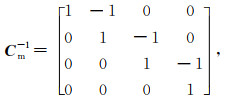
附录此附录针对正文中单方法和联合反演目标函数的模型项中Cm-1、Cm1/2、Cm-1/2进行简要说明.常规而言,Cm-1一般是一阶/二阶平滑或者拉普拉斯平滑,我们以一维方向4个模型参数来简要说明.根据一阶平滑计算公式,Cm-1可以写成:
|
(A1) |
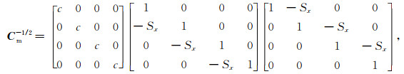
而采用Cm-1/2、Cm1/2平滑方法,其变换公式为
|
(A2) |
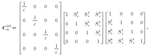
|
(A3) |
其中Sx为沿x轴方向的平滑因子,c=1/(1-Sx)2.
在三维模型中,Cm-1/2和Cm1/2应用思路为:分别对每个方向(x、y、z)的光滑因子Sx、Sy、Sz,然后三个方向分别进行公式(F2、F3)的光滑处理,在Egbert和Kelbert(2012)的光滑策略中,还可以选择每个方向的光滑次数,次数越多,模型就越光滑.本文中选取Sx=Sy=Sz=0.2,光滑两次,或者Sx=Sy=Sz=0.5,光滑一次.
致谢 感谢两位评审专家在百忙之中为本文的修改提出细致而宝贵的意见.
Abubakar A, Gao G, Habashy T M, et al. 2012. Joint inversion approaches for geophysical electromagnetic and elastic full-waveform data. Inverse Problems, 28(5): 055016. DOI:10.1088/0266-5611/28/5/055016 |
Arie K, Adam A, Smythe D K. 1997. Combined seismic and magnetotelluric imaging of upper crystalline crust in the southern Bohemian massif. First Break, 15(8): 265-271. DOI:10.1046/j.1365-2397.1997.00670.x |
Barde-Cabusson S, Bolós X, Pedrazzi D, et al. 2013. Electrical resistivity tomography revealing the internal structure of monogenetic volcanoes. Geophysical Research Letters, 40(11): 2544-2549. DOI:10.1002/grl.50538 |
Bennington N L, Zhang H J, Thurber C H, et al. 2015. Joint inversion of seismic and magnetotelluric data in the parkfield region of california using the normalized cross-gradient constraint. Pure and Applied Geophysics, 172(5): 1033-1052. |
Berdichevsky M N, Dmitriev V I. 2008. Models and Methods of Magnetotellurics. Berlin Heidelberg: Springer.
|
Byrd R H, Nocedal J, Schnabel R B. 1994. Representations of quasi-newton matrices and their use in limited memory methods. Mathematical Programming, 63(1): 129-156. |
Chen X, Yu P, Zhang L L, et al. 2010. Regularized synchronous joint inversion of MT and seismic data. Seismology and Geology (in Chinese), 32(3): 402-408. |
Chen X, Yu P, Deng J Z, et al. 2016. Joint inversion of MT and seismic data based on wide-range petrophysical constraints. Chinese Journal of Geophysics (in Chinese), 59(12): 4690-4700. DOI:10.6038/cjg20161228 |
Colombo D, De Stefano M. 2007. Geophysical modeling via simultaneous joint inversion of seismic, gravity, and electromagnetic data:Application to prestack depth imaging. The Leading Edge, 26(3): 326-331. |
Demirci I, Candansayar M E, Vafidis A, et al. 2017. Two dimensional joint inversion of direct current resistivity, radio-magnetotelluric and seismic refraction data:An application from Bafra Plain, Turkey. Journal of Applied Geophysics, 139: 316-330. DOI:10.1016/j.jappgeo.2017.03.002 |
Dobróka M, Gyulai Á, Ormos T, et al. 1991. Joint inversion of seismic and geoelectric data recorded in an underground coal mine. Geophysical Prospecting, 39(5): 643-665. DOI:10.1111/j.1365-2478.1991.tb00334.x |
Egbert G D, Kelbert A. 2012. Computational recipes for electromagnetic inverse problems. Geophysical Journal International, 189(1): 251-267. DOI:10.1111/j.1365-246X.2011.05347.x |
Fang H J, Yao H J, Zhang H J, et al. 2015. Direct inversion of surface wave dispersion for three-dimensional shallow crustal structure based on ray tracing:methodology and application. Geophysical Journal International, 201(3): 1251-1263. DOI:10.1093/gji/ggv080 |
Gallardo L A, Meju M A. 2003. Characterization of heterogeneous near-surface materials by joint 2D inversion of dc resistivity and seismic data. Geophysical Research Letters, 30(13): 1658. DOI:10.1029/2003GL017370 |
Gallardo L A, Meju M A. 2004. Joint two-dimensional DC resistivity and seismic travel time inversion with cross-gradients constraints. Journal of Geophysical Research:Solid Earth, 109(B3): B03311. DOI:10.1029/2003JB002716 |
Gallardo L A. 2007a. Multiple cross-gradient joint inversion for geospectral imaging. Geophysical Research Letters, 34(19): L19301. DOI:10.1029/2007GL030409 |
Gao J, Zhang H J. 2016. Two-dimensional joint inversion of seismic velocity and electrical resistivity using seismic travel times and full channel electrical measurements based on alternating cross-gradient structural constraint. Chinese Journal of Geophysics (in Chinese), 59(11): 4310-4322. DOI:10.6038/cjg20161131 |
Gao J, Zhang H J, Fang H J, et al. 2017. An efficient joint inversion strategy for 3D seismic travel time and DC resistivity data based on cross-gradient structure constraint. Chinese Journal of Geophysics (in Chinese), 60(9): 3628-3641. DOI:10.6038/cjg20170927 |
Gao R. 1995. A review of the results of geophysical investigation of the crust and upper mantle in the Qinghai Tibet Plateau. Chinese Geology, (4): 26-28. |
Hauck C. 2002. Frozen ground monitoring using DC resistivity tomography. Geophysical Research Letters, 29(21): 12-1. |
Hu W Y, Abubakar A, Habashy T M. 2009. Joint electromagnetic and seismic inversion using structural constraints. Geophysics, 74(6): R99-R109. DOI:10.1190/1.3246586 |
Infante V, Gallardo L A, Montalvo-Arrieta J C, et al. 2010. Lithological classification assisted by the joint inversion of electrical and seismic data at a control site in northeast Mexico. Journal of Applied Geophysics, 70(2): 93-102. DOI:10.1016/j.jappgeo.2009.11.003 |
Jing R Z, Bao G S, Chen S Q. 2003. A review of the researches for geophysical combinative inversion. Progress in Geophysics (in Chinese), 18(3): 535-540. |
Jones F W, Pascoe L J. 1971. A general computer program to determine the perturbation of alternating electric currents in a two-dimensional model of a region of uniform conductivity with an embedded inhomogeneity. Geophysical Journal of the Royal Astronomical Society, 24(1): 3-30. DOI:10.1111/j.1365-246X.1971.tb01844.x |
Krautblatter M, Hauck C. 2007. Electrical resistivity tomography monitoring of permafrost in solid rock walls. Journal of Geophysical Research:Earth Surface, 112(F2): F02S20. DOI:10.1029/2006JF000546 |
Li H Y, Su W, Wang C Y, et al. 2009. Ambient noise Rayleigh wave tomography in western Sichuan and eastern Tibet. Earth and Planetary Science Letters, 282(1-4): 201-211. DOI:10.1016/j.epsl.2009.03.021 |
Li H Y, Song X D, Lv Q T, et al. 2019. Seismic imaging of lithosphere structure and upper mantle deformation beneath east-central China and their tectonic implications. Journal of Geophysical Research:Solid Earth, 123(4): 2856-2870. |
Li S C, Nie L C, Liu B, et al. 2015. Advanced detection and physical model test based on multi-electrode sources array resistivity method in tunnel. Chinese Journal of Geophysics (in Chinese), 58(4): 1434-1446. DOI:10.6038/cjg20150429 |
Li T L, Zhang R Z, Pak Y. 2015. Joint inversion of magnetotelluric and first-arrival wave seismic traveltime with cross-gradient constraints. Journal of Jilin University (Earth Science Edition) (in Chinese), 45(3): 952-961. |
Li Z X, Tan H D, Fu S S, et al. 2015. Two-dimensional synchronous inversion of TDIP with cross-gradient constraint. Chinese Journal of Geophysics (in Chinese), 58(12): 4718-4726. DOI:10.6038/cjg20151232 |
Linde N, Binley A, Tryggvason A, et al. 2006. Improved hydrogeophysical characterization using joint inversion of cross-hole electrical resistance and ground-penetrating radar traveltime data. Water Resources Research, 42(12): W12404. DOI:10.1029/2006WR005131 |
Lv Q T, Dong S W, Tang J T, et al. 2015. Multi-scale and integrated geophysical data revealing mineral systems and exploring for mineral deposits at depth:A synthesis from SinoProbe-03. Chinese Journal of Geophysics (in Chinese), 58(12): 4319-4343. DOI:10.6038/cjg20151201 |
Ma H, Guo Y, Wu P P, et al. 2018. 3-D joint inversion of multi-array data set in the resistivity method based on MPI parallel algorithm. Chinese Journal of Geophysics (in Chinese), 61(12): 5052-5065. DOI:10.6038/cjg2018M0005 |
Molodtsov D M, Troyan V N, Roslov Y V, et al. 2013. Joint inversion of seismic traveltimes and magnetotelluric data with a directed structural constraint. Geophysical Prospecting, 61(6): 1218-1228. DOI:10.1111/1365-2478.12060 |
Moorkamp M, Heincke B, Jegen M, et al. 2011a. A framework for 3-D joint inversion of MT, gravity and seismic refraction data. Geophysical Journal International, 184(1): 477-493. DOI:10.1111/j.1365-246X.2010.04856.x |
Newman G A, Gasperikova E, Hoversten G M, et al. 2008. Three-dimensional magnetotelluric characterization of the Coso geothermal field. Geothermics, 37(4): 369-399. DOI:10.1016/j.geothermics.2008.02.006 |
Peng M, Tan H D, Jiang M, et al. 2013. Three-dimensional joint inversion of magnetotelluric and seismic travel time data with cross-gradient constraints. Chinese Journal of Geophysics (in Chinese), 56(8): 2728-2738. DOI:10.6038/cjg20130821 |
Peng M, Tan H D, Moorkamp M. 2019. Structure-coupled 3-D imaging of magnetotelluric and wide-angle seismic reflection/refraction data with interfaces. Journal of Geophysical Research:Solid Earth, 124(10): 10309-10330. DOI:10.1029/2019JB018194 |
Roux P, Sabra K G, Kuperman W A, et al. 2005. Ambient noise cross correlation in free space:Theoretical approach. The Journal of the Acoustical Society of America, 117(1): 79-84. DOI:10.1121/1.1830673 |
Shapiro N M, Campillo M, Stehly L, et al. 2005. High-resolution surface-wave tomography from ambient seismic noise. Science, 307(5715): 1615-1618. DOI:10.1126/science.1108339 |
Shi Z J, Hobbs R W, Moorkamp M, et al. 2017. 3-D cross-gradient joint inversion of seismic refraction and DC resistivity data. Journal of Applied Geophysics, 141: 54-67. DOI:10.1016/j.jappgeo.2017.04.008 |
Tang J T, Zhang J F, Feng B, et al. 2007. Determination of borders for resistive oil and gas reservoirs by deviation rate using the hole-to-surface resistivity method. Chinese Journal of Geophysics (in Chinese), 50(3): 926-931. |
Um E S, Commer M, Newman G A. 2014. A strategy for coupled 3D imaging of large-scale seismic and electromagnetic data sets:Application to subsalt imaging. Geophysics, 79(3): ID1-ID13. |
Vozoff K, Jupp D L B. 1975. Joint inversion of geophysical data. Geophysical Journal of the Royal Astronomical Society, 42(3): 977-991. |
Weaver R L. 2005. Information from Seismic Noise. Science, 307(5715): 1568-1569. DOI:10.1126/science.1109834 |
Wu P P, Tan H D, Lin C H, et al. 2020. Joint inversion of two-dimensional magnetotelluric and surface wave dispersion data with cross-gradient constraints. Geophysical Journal International, 221(2): 938-950. DOI:10.1093/gji/ggaa045 |
Wu X P, Xu G M. 2000. Study on 3-D resistivity inversion using conjugate gradient method. Chinese Journal of Geophysics (in Chinese), 43(3): 420-427. |
Wu X P, Wang T T. 2001. Study on some problems for 3D resistivity inversion using conjugate gradient. Seismology and Geology (in Chinese), 23(4): 321-327. |
Yan Z W, Tan H D, Peng M, et al. 2020. Three-dimensional joint inversion of gravity, magnetic and magnetotelluric data based on cross-gradient theory. Chinese Journal of Geophysics (in Chinese), 63(2): 736-752. DOI:10.6038/cjg2020M0355 |
Yang H, Dai S K, Song H B, et al. 2002. Overview of joint inversion of integrated geophysics. Progress in Geophysics (in Chinese), 17(2): 262-271. |
Yang Z W, Wang J Y, Zhang S Y, et al. 1998. Research on joint inversion of 1-D magnetotelluric and seismic data. Oil Geophysical Prospecting (in Chinese), 33(1): 78-88. |
Yao H J, Van Der Hilst R D, De Hoop M V. 2006. Surface-wave array tomography in SE Tibet from ambient seismic noise and two-station analysis-I. Phase velocity maps. Geophysical Journal International, 166(2): 732-744. |
Yao H J, Beghein C, Van Der Hilst R D. 2008. wave array tomography in SE Tibet from ambient seismic noise and two-station analysis-Ⅱ. Crustal and upper-mantle structure. Geophysical Journal of the Royal Astronomical Society, 173(1): 205-219. DOI:10.1111/j.1365-246X.2007.03696.x |
Yu P, Dai M G, Wang J L, et al. 2009. Joint inversion of magnetotelluric and seismic data based on random resistivity and velocity distributions. Chinese Journal of Geophysics (in Chinese), 52(4): 1089-1097. |
Yuval D, Oldenburg W. 1996. DC resistivity and IP methods in acid mine drainage problems:results from the Copper Cliff mine tailings impoundments. Journal of Applied Geophysics, 34(3): 187-198. DOI:10.1016/0926-9851(95)00020-8 |
Zhang R Z, Li T L, Deng H, et al. 2019. 2D joint inversion of MT, gravity, magnetic and seismic first-arrival wave traveltime with cross-gradient constraints. Chinese Journal of Geophysics (in Chinese), 62(6): 2139-2149. DOI:10.6038/cjg2019L0713 |
陈晓, 于鹏, 张罗磊, 等. 2010. 大地电磁与地震正则化同步联合反演. 地震地质, 32(3): 402-408. |
陈晓, 于鹏, 邓居智, 等. 2016. 基于宽范围岩石物性约束的大地电磁和地震联合反演. 地球物理学报, 59(12): 4690-4700. DOI:10.6038/cjg20161228 |
高级, 张海江. 2016. 基于交叉梯度交替结构约束的二维地震走时与全通道直流电阻率联合反演. 地球物理学报, 59(11): 4310-4322. DOI:10.6038/cjg20161131 |
高级, 张海江, 方洪健, 等. 2017. 一种高效的基于交叉梯度结构约束的三维地震走时与直流电阻率联合反演策略. 地球物理学报, 60(9): 3628-3641. DOI:10.6038/cjg20170927 |
高锐. 1995. 青藏高原地壳上地幔地球物理调查研究成果综述(上). 中国地质, (4): 26-28. |
敬荣中, 鲍光淑, 陈绍裘. 2003. 地球物理联合反演研究综述. 地球物理学进展, 18(3): 535-540. |
李术才, 聂利超, 刘斌, 等. 2015. 多同性源阵列电阻率法隧道超前探测方法与物理模拟试验研究. 地球物理学报, 58(4): 1434-1446. DOI:10.6038/cjg20150429 |
李桐林, 张镕哲, 朴英哲. 2015. 大地电磁测深与地震初至波走时交叉梯度反演. 吉林大学学报(地球科学版), 45(3): 952-961. |
李兆祥, 谭捍东, 付少帅, 等. 2015. 基于交叉梯度约束的时间域激发极化法二维同步反演. 地球物理学报, 58(12): 4718-4726. DOI:10.6038/cjg20151232 |
吕庆田, 董树文, 汤井田, 等. 2015. 多尺度综合地球物理探测:揭示成矿系统、助力深部找矿——长江中下游深部探测(SinoProbe-03)进展. 地球物理学报, 58(12): 4319-4343. DOI:10.6038/cjg20151201 |
马欢, 郭越, 吴萍萍, 等. 2018. 基于MPI并行算法的电阻率法多种装置数据的三维联合反演. 地球物理学报, 61(12): 5052-5065. DOI:10.6038/cjg2018M0005 |
彭淼, 谭捍东, 姜枚, 等. 2013. 基于交叉梯度耦合的大地电磁与地震走时资料三维联合反演. 地球物理学报, 56(8): 2728-2738. DOI:10.6038/cjg20130821 |
汤井田, 张继锋, 冯兵, 等. 2007. 井地电阻率法歧离率确定高阻油气藏边界. 地球物理学报, 50(3): 926-931. |
吴小平, 徐果明. 2000. 利用共轭梯度法的电阻率三维反演研究. 地球物理学报, 43(3): 420-427. |
吴小平, 汪彤彤. 2001. 利用共轭梯度方法的电阻率三维反演若干问题研究. 地震地质, 23(2): 321-327. |
闫政文, 谭捍东, 彭淼, 等. 2020. 基于交叉梯度约束的重力、磁法和大地电磁三维联合反演. 地球物理学报, 63(2): 736-752. DOI:10.6038/cjg2020M0355 |
杨辉, 戴世坤, 宋海斌, 等. 2002. 综合地球物理联合反演综述. 地球物理学进展, 17(2): 262-271. |
杨振武, 王家映, 张胜业, 等. 1998. 一维大地电磁和地震数据联合反演方法研究. 石油地球物理勘探, 33(1): 78-88. |
于鹏, 戴明刚, 王家林, 等. 2009. 电阻率和速度随机分布的MT与地震联合反演. 地球物理学报, 52(4): 1089-1097. |
张镕哲, 李桐林, 邓海, 等. 2019. 大地电磁、重力、磁法和地震初至波走时的交叉梯度二维联合反演研究. 地球物理学报, 62(6): 2139-2149. DOI:10.6038/cjg2019L0713 |