2018年8月19日00时19分36秒(UTC)，在斐济东部海域(178.11°W, 18.18°S)发生了一次M_W8.2级地震(斐济M_W8.2地震)，震源深度达563 km.这是继1994年玻利维亚M_W8.2深震(震源深度637 km)(Wiens et al., 1994; Chen, 2013; Zhan et al., 2014)以及2013年鄂霍茨克海M_W8.3深震(震源深度607 km)(Meng et al., 2014; Zhan et al., 2014)之后又一次深源大地震.

深源地震的震源与浅源地震在很多方面都具有相似性(Wiens, 1998, 2001)，其中最为突出的特点就是深源地震的震源机制可以近似为一个双力偶表示的平面错动，非双力偶成分占比很小(Kikuchi and Kanamori, 2013; Zhan et al., 2014).这清楚地表明深源地震仍属平面错动.

根据美国地质调查局(USGS)和全球矩心矩张量(GCMT)解(表 1)，斐济M_W8.2地震的正断层分量占绝对优势.截至北京时间2018年8月20日9时50分, 在震中区附近(16.8°S—18.8°S，179°W—177.2°W)共记录到34次4.2级以上余震，震源深度分布在399~641 km之间.其中最大一次余震的震级为M_W6.8，震源深度为415 km，但逆断层分量占绝对优势(图 1a).

表 1 (Table 1)

表 1 斐济MW8.2深震震源机制解 Table 1 Focal mechanism solutions of the Fiji MW8.2 deep earthquake Sources Scalar Moment(N-m) Depth/km Plane Ⅰ Plane Ⅱ Strike/(°) Dip/(°) Rake/(°) Strike /(°) Dip/(°) Rake /(°) GCMT 2.630×1021 555 210 21 -74 13 70 -96 USGS 2.553×1021 558.6 209 21 -79 18 69 -94

表 1 斐济MW8.2深震震源机制解 Table 1 Focal mechanism solutions of the Fiji MW8.2 deep earthquake

图 1

Fig. 1

图 1 2018年斐济MW8.2地震及其较大余震(Mb>4.2)震中位置以及阿拉斯加地震台网台站分布 (a)主震及其较大余震的震中分布.两个青色的海滩球分别表示主震和最大余震(MW6.8)的震源机制(来自：美国地质调查局)，红色沙滩球表示主震GCMT震源机制解；(b)主震和台阵的相对位置；(c)阿拉斯加地震台网台站的分布，其中红色台站被用做参考台. Fig. 1 Map showing epicenters of the 2018 MW8.2 Fiji earthquake and its major aftershocks (Mb>4.2) and the Alaska seismograph network (a) Epicenters of the main earthquake and major aftershocks. The USGS focal mechanism solutions of the main shock and its largest aftershock (MW6.8) are in cyan while the GCMT solution of the main shock is in red; (b) The relative locations of the array with respect to the main earthquake; (c) Station distribution of the Alaska seismograph network, where the red station is used as the reference station.

关于深源地震的成因或发生机理，一直是地震学研究的热点之一，也取得了一些认识，例如：热剪切失稳(Thermal shear instability)(Ogawa, 1987; Kikuchi and Kanamori., 2013; Silver et al., 1995; Kanamori et al., 1998; Karato et al., 2015; Zhan et al., 2014; Zhan, 2017), 脱水脆化(Dehygration embrittlement)(Meade and Jeanloz, 1991; Silver et al., 1995; Jung et al., 2004), 过渡性断裂(Transformational faulting)(Kirby, 1996; Frohlich, 1989; Green II and Burnley, 1989; Green II et al., 2015; Kirby et al., 1991; Wiens et al., 1994; Green II, 1993; Marone and Liu, 2013; Zhao, 2017; 王曙光等，2011), 还有锁固段模型(吴晓娲等, 2016).但仍无定论(Chen, 2013; 干微等，2012; Goes and Ritsema, 2013; Meng et al., 2014).

现代地震学理论、方法和技术的发展，虽然还不能直接回答有关深源地震成因或发生机理的问题，但其观测结果为回答这些问题可以提供有效的物理约束(Wiens, 2001; Tibi et al., 2003).远场台阵反投影技术就是近年来发展起来且经大量应用被广泛认可的观测震源破裂过程的一种有效方法(Ishii et al., 2005; Krüger and Ohrnberger, 2005; Lay et al., 2017)，且由此产生了许多与此类似的技术及其应用(Ishii et al., 2007; Walker and Shearer, 2009; Meng et al., 2011, 2012; Yagi et al., 2012; Yao et al., 2013; Zhang et al., 2012; Xu et al., 2013; Qin and Yao, 2017; Yin et al., 2017; Wang and Mori, 2016; Meng et al., 2016; 王晓欣等，2017; 刘志鹏等，2018).自2004年苏门答腊大地震发生以来，我们曾多次利用这种方法对一些重要地震的破裂过程进行过研究(杜海林，2007; 许力生等，2008; 杜海林等，2009; Zhang et al., 2009; 杜海林和许力生，2012), 注意到这种方法可以较客观地揭示地震破裂的轨迹、破裂的尺度以及破裂的速度等.

2018年8月19日斐济M_W8.2地震发生后，位于美国阿拉斯加的宽频带地震台站记录到了这次地震.如图 1b所示，这些台站距离震中在77.9°和89.4°之间，为利用反投影技术确定地震的破裂轨迹、破裂尺度以及破裂速度提供了良好的机会.这里将展示对这次地震的分析结果，并对可能的发震机理提出自己的看法.

经典的台阵技术多种多样(Rost and Thomas, 2002)，但近年来被广泛采用的技术多来源于Ishii等(2005)以及Krüger和Ohrnberger(2005)采用的广义反投影技术.简而言之，首先对台阵所有记录初动进行走时校正，使其与理论走时一致，然后对所有记录进行多次幂聚束叠加，最后通过叠加能量的对比得到破裂点的位置和时间.

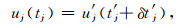
若用u′_j(t′_j)表示台阵中第j个台站的归一化记录, 用u_j(t_j)表示走时校正后的记录，则：

(1)

这里δt′_j是观测走时与理论走时之差.

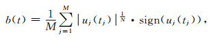
如果对台阵中的M个台站的信号进行1/N次幂叠加，则聚束信号可表示为(Rost and Thomas, 2002; Xu et al., 2013)

(2)

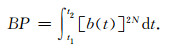
那么，聚束信号在时间t₁~t₂之间的能量为

(3)

通常情况下N取4(Xu et al., 2013; Yagi et al., 2012; Honda et al., 2013)，对原始信号进行非线性处理.但对于此次事件，选用的信号质量相对较高，无须进行非线性处理，所以在此取N=1.

反投影技术可以根据不同情况利用多种震相(Kiser et al., 2011; Koper et al., 2012; Roten et al., 2012; Jian et al., 2017), 但P震相具有频率相对高且因最先到达而不易受其他震相干扰等优点(Ishii et al., 2005)，因此本文仍采用P波.

我们从IRIS数据中心下载了震中距在30°~90°的所有宽频带记录的垂直分量.根据经验用信噪比阈值10以及P波段(t_p~t_p+35 s)相关系数阈值0.75去优选数据，最终选定如图 1b所示的位于美国阿拉斯加的北美移动台阵(TA)的131个台站.这些台站的震中距在77.9°和89.4°之间，方位角在4.69°与24.55°之间.

为了确保反投影结果的初始破裂点与已经发布的仪器震源位置一致，首先采用改进自杜海林(杜海林，2007)的互相关技术，依据ak135速度模型(Kennett et al., 1995)对原始记录(图 2a)的P波到时进行了校正.

图 2

Fig. 2

图 2 主震的观测数据 (a)原始地震记录的垂直分量(P波前10 s，P波后50 s)，红色竖线表示P波理论到时; (b)原始记录的振幅归一化振幅谱，所选频段上下限分别用蓝色和红色竖线表示；(c)所选频段的地震记录. Fig. 2 Observational data of the main shock (a) The vertical components of raw records (10 s before and 50 s after P arrivals). Red vertical line indicates the theoretical arrival time of P-waves; (b) The amplitude-normalized spectrum of raw records. Upper and lower frequency limits are shown with blue and red vertical lines, respectively; (c) Band-pass filtered seismic records.

为了获得携带震源破裂信息的频段，首先计算了60 s(初动前后分别为10 s和50 s)时长的P波段振幅谱(图 2b), 并根据振幅谱的特征选定了0.5~2 Hz的频带.与此同时，为了了解这个频段内的台阵响应，分别在0.5 Hz、1 Hz和2 Hz计算了台阵响应.如图 3所示，即使在2 Hz的高频, 台阵响应函数仍呈清晰的单峰，因此采用了0.5~2 Hz的3阶巴特沃斯带通滤波器对原始记录进行了滤波，得到如图 2c所示的P波段高频记录，以备反投影使用.

图 3

Fig. 3

图 3 阿拉斯加台阵在斐济MW8.2地震震中位置的台阵响应 (a)在0.5 Hz; (b)在1 Hz; (c)在2 Hz.红色五角星表示主震震中位置. Fig. 3 The response of the Alaska array at the epicenter of the 2018 MW8.2 Fiji earthquake (a) At 0.5 Hz; (b) At 1 Hz; (c) At 2 Hz. Red star is epicenter location.

投影的目标区确定为16.8°S—18.8°S和179°W—177.2°W之间，并按0.005°的间隔将目标区分成361×401个网格.根据对校正后首个滑动时窗内所有波形相关度以及分辨尺度的折衷，最终采用了5 s的时间窗和0.2 s的移动步长.图 4选择性地展示了其中6个时间窗的能量分布，由此可以看出高频能量随时间和空间的变迁.

图 4

Fig. 4

图 4 不同时窗内聚束能量的空间分布 其中五角星表示破裂起始点(仪器震中)，红色圆圈表示瞬时能量最大点. Fig. 4 Spatial distribution of the beam energy within various time windows Red stars are the initial points (instrument epicenters) and red circles denote the points of the maximal instantaneous energy.

为了确定这次地震的有效破裂时间，我们采用了早期提出的判据(杜海林, 2007; 杜海林等，2009).根据这个判据，分别计算聚束波形与参考波形的振幅比随时间的变化、聚束波形与参考波形的相关系数随时间的变化以及聚束能量随时间的变化，然后由它们的点积确定所谓γ函数，此函数的有效持续时间被当作破裂的有效持续时间.如图 5d所示，此次地震的有效持续时间可确定为22 s.

图 5

Fig. 5

图 5 有效持续时间的确定 (a)聚束波形与参考波形的相关系数；(b)聚束波形与参考波形的振幅比；(c)聚束能量；(d)有效持续时间的判据函数，衰减至γ函数最大幅值2%的时刻为有效持续时间. Fig. 5 Determination of the effective duration time (a) Correlation coefficient between beam-formed waveforms data and reference waveforms; (b) Amplitude ratio of beam-formed waveforms to reference waveforms; (c) Radiation energy; (d) Criterion function of the effective duration. The effective duration is the time at which the amplitude of gamma function drops to 2%.

在目标区为每一个时间点或时间窗获取一个能量最大的位置便可以得到如图 6a所示的图像.这个图像清楚地展示了高频辐射源随时间和空间的变化.粗略地看，这是一个简单的单侧破裂，破裂从仪器震源位置开始，逐渐向近北方向传播，破裂到北端略有回折并结束.

图 6

Fig. 6

图 6 高频源时空过程与破裂方位 (a)高频源时空过程，红色六芒星为起始点，彩色圆圈表示高频源瞬时位置，圆圈大小表示能量相对大小, 红色沙滩球为GCMT给出的震源机制解，蓝色沙滩球为USGS发布的震源机制解，白色六芒星为34个余震的位置；(b)破裂方向的估计, 圆圈大小表示能量相对大小，图例中两个距离分别为最远破裂距离以及最高能量释放位置处的距离，黑色实线为最高能量释放位置相对于初始破裂点的方位角，红色虚线为根据最小二乘估计的平均方位角. Fig. 6 Spatio-temporal process of high-frequency sources and the azimuth estimation of the rupture (a) The spatio-temporal process of the high-frequency sources. The red beach ball is the focal mechanism solutions given by GCMT, the blue beach ball is the focal mechanism solutions issued by USGS, and the white hexagram indicates the aftershock locations; (b) The azimuth estimation of the rupture. In the legend, the two distances, from the furthest location and the energy-highest location, are presented. The black solid line points to the azimuth of the energy-highest location while the red dash line shows the average of the azimuths based on the least-squared estimation.

为了确定破裂方向与尺度，我们将破裂前锋位置投影到如图 6b所示的极坐标系中，其径向方向为破裂点距初始点的距离，切向方向为方位角.从图中可以看出，破裂从震源位置(178.11°W，18.18°S)开始，总体向近北方向扩展，但瞬时方位随时间和空间有所变化.根据计算，能量最大点相对于初始破裂点的方位为2.3°.基于最小二乘方法对整个过程的平均破裂方向进行最优估计，其方位约3.0°.根据计算，能量最大点距离初始破裂点40 km，而如果把整个破裂过程中最远破裂点距初始破裂点的距离作为震源破裂尺度，则约为51 km.

为了确定破裂速度，我们将破裂前锋位置投影到“时间-距离”直角坐标系中.如图 7所示，破裂点距起始点的距离总体上随时间逐渐增加，但也不是线性递增.为此利用最小二乘法为这次地震估计了4个破裂速度.第一个为能量最大点即约15 s(14.6 s)(图 7a)之前的平均破裂速度，第二个为整个过程即0~22 s内的平均破裂速度，第三个破裂速度为第一次子事件(0~10 s)的破裂速度，第四个破裂速度为第二次子事件(10~22 s)的平均破裂速度.如图 7b所示，得到的速度分别为2.7 km·s^-1、2.5 km·s^-1、2.9 km·s^-1和1.6 km·s^-1.这几个破裂速度均小于震源周围的S波速度~5.4 km·s^-1.

图 7

Fig. 7

图 7 辐射能量随时间的变化与破裂速度估计 (a)有效破裂时间内辐射能量随时间的变化.最大峰值出现在14.6(~15)s；(b)破裂速度的估计.黑色虚线为最高能量位置之前的破裂速度，红色虚线为全过程平均速度, 绿色虚线为0~10 s平均破裂速度，蓝色虚线为10~22 s平均破裂速度. Fig. 7 Temporal variation of radiation energy and the estimation of rupture velocity (a) The temporal variation of the radiation energy during the effective duration. The maximum of the energy appears at 14.6 s(~15 s); (b) The estimation of rupture velocity. The black dash line is the rupture velocity before the energy-highest time, red dash line is the average velocity over the entire process, green dash line is the average velocity in the first ~10 s, and blue dash line is average velocity in the period of 10~22 s.

对比GCMT和USGS分别给出的震源机制解的两个节面参数(表 1)，我们相信两者的第二个节面(走向：13°；走向：18°)更接近真实的发震断层面(图 8)，总体倾角很陡，向近东倾斜，东侧物质相对下移，形成正断层运动.

图 8

Fig. 8

图 8 1990—2018年之间震中区地震(M≥5.5)的空间分布 (a)地震在水平面上的分布；(b)图(a)中ABCD方框内地震在EF剖面上的投影.青色海滩球表示主震的震源机制，红色五角星表示主震的位置，红色直线表示USGS给出的断层面NPII(18°/69°/-94°)，彩色圆表示历史地震位置，颜色表示深度，半径表示相对大小. Fig. 8 Spatial distribution of the 1990—2018 earthquakes (M≥5.5) around the epicenter area (a) The map view of hypocenters; (b) The projection on the cross-section along the line EF of the hypocenters in the frame ABCD shown in (a). The cyan beach-balls are focal mechanism solutions of the main shock, the red star denotes the location of the main shock, red lines crossing the stars represent the nodal plane (NPII: 18°/69°/-94°) given by USGS, the color-filled circles display the hypocenters where color indicates depth and radius shows the relative size.

深源地震的尺度和方向为孕震带的形状和空间提供了一定的约束，进而为可能的错断模型提供约束(Tibi et al., 2003).对于大多数深源地震而言，破裂发生在一个平行于地震带走向的很窄的一个条带内，但也有少数例外.例如，1994年玻利维亚地震和1994年斐济—汤加地震，发震断层垂直切入俯冲板块(Goes and Ritsema, 2013; McGuire et al., 1997; Zhan et al., 2014).2018年斐济M_W8.2地震的破裂方向基本沿着俯冲板块的走向，属于第一种类型.

深源地震的破裂速度是板块温度的函数，其变化范围大多数在震源处剪切波速度的30%~90%之间(Tibi et al., 2003).观测表明冷板块中破裂速度较大，而热板块中破裂速度较小(Wiens, 1998, 2001; Tibi et al., 1999).2018年斐济M_W8.2地震的破裂速度在震源处剪切波速度的48%~50%之间，相当于已有深源地震破裂速度的中间值(Tibi et al., 2003).

深源地震的地震效率也是随板块的温度发生变化的(Tibi et al., 2003, Venkataraman and Kanamori, 2004)，大多数地震的地震效率在25%~100%之间，但也有一些地震的地震效率非常低, 例如1994年的玻利维亚地震(Kikuchi and Kanamori, 2013)以及1999年的中苏边界地震(Tibi et al., 2003; Venkataraman and Kanamori, 2004).对于深源地震，效率较高的地震发生在较冷的板块内部，而效率较低的地震发生在较热的板块内部.地震效率可以用断层的临界位错和平均位错估计(Olsen et al., 1997；Guatteri and Spudich, 2000)，也可以用辐射能量、应力降和标量地震矩估计(Kanamori et al., 1998; Venkataraman and Kanamori, 2004; Kanamori and Brodsky, 2001)，还可以用破裂速度加以估计(Kanamori et al., 1998; Venkataraman and Kanamori, 2004; Kanamori and Brodsky, 2001).尽管由于每个参数测量的不确定性，用不同的方法估计的同一个地震的地震效率之间存在差异，但不同方法得到的一组地震的趋势性特征是一致的(Venkataraman and Kanamori, 2004; Kanamori and Brodsky, 2001).对于2018年斐济M_W8.2地震，基于Ⅲ型裂纹的假设直接利用破裂速度计算了辐射效率.前15 s的辐射效率为42%，整个过程的辐射效率约为39%，然而第一次子事件(前10 s)的辐射效率为45%，第二次子事件(10~22 s)效率骤降至26%.

根据脱水脆化破裂机制，脱水过程产生的水增加了孔隙压，减小了正应力，从而引起脆性破裂.这种机理多用来解释下地壳到地幔最顶部的中深源地震(Frohlich, 1989; Green II, 1993; Kirby et al., 1996; Tibi et al., 2003).根据过渡性断裂机制，板块内部发生相变，产生不连续性，进而产生断层发生地震.这种机制主要用来解释地幔过渡带发生的地震(Kirby, 1991).根据剪切失稳机制，在俯冲板块的深部，沿着剪切带的温度由于黏性耗散可能会突然增加，这种温度的突然增加会引起熔融，由此会产生沿着剪切带的滑动(Griggs and Baker, 1968; Ogawa, 1987; Hobbs and Ord, 1988).破裂一旦开始，由于阻力而出现熔融，滑动继续，但由于熔融，应变能转化成热能得以耗散，地震效率降低，破裂速度变小，最终破裂停止(Kanamori et al., 1998).

如图 8所示，2018年斐济M_W8.2地震发生在近600 km的俯冲板块的最前缘，且震源周围已有大量地震分布在较大的空间范围内，这表明陆壳下插受到阻力，且阻力随深度增加而增加，形成如图中箭头所示的剪切作用，断层下盘(较深段)受到高温物质的上浮阻力而相对上滑，形成正断层.地震的断层面平行于俯冲板块的走向，破裂沿走向单侧传播，形成典型的横向剪切裂纹(Transverse shear crack)或者Ⅲ型裂纹(Crack Mode Ⅲ)(Venkataraman and Kanamori, 2004; Kanamori and Brodsky, 2001).由于深达近600 km的地幔深处不具备脱水脆化的可能(Kirby et al., 1996；Tibi et al., 2003)，因此2018年斐济M_W8.2地震的开始很可能源于相变或过渡性断裂(Kirby et al., 1991, 1996).破裂开始后，冷剪切发挥主导作用，破裂速度较快，辐射效率较高，因此，第一次事件的破裂速度达到2.9 km·s^-1，辐射效率为45%.随后由于热耗散作用，热剪切和熔融发挥主导作用，破裂速度减小，辐射效率减低，因此，第二次事件的破裂速度减小到1.6 km·s^-1，辐射效率降至26%.跟1994年玻利维亚地震不同(Zhan et al., 2014)，2018年斐济M_W8.2地震整个破裂过程都在沿俯冲板块的走向进行，辐射效率约40%，属于典型的俯冲板块“冷”环境下发生的深源地震(Wiens, 2001; Venkataraman and Kanamori, 2004; Ye et al., 2013, 2016a, b).

简而言之，2018年斐济M_W8.2地震在深达近600 km的高温高压环境下，由于俯冲板块的顶部受到较大上浮阻力形成剪切作用，很可能由于板块内部的相变作用使地震成核，进而发生剪切失稳，形成横向剪切形成了正断层错动.

2018年斐济M_W8.2地震是一次单侧破裂事件，总体破裂方位在3.0°左右，持续时间22 s，破裂长度达~51 km，平均破裂速度为2.5 km·s^-1.能量释放有2次高峰，形成两次子事件.第一次发生在前10s，破裂速度为2.9 km·s^-1，辐射效率为45%.第二次为10~22 s，破裂速度为1.6 km·s^-1，辐射效率为26%.这次地震的发生很可能源于俯冲板块前缘受到下部地幔物质上浮阻力引起的剪切失稳.起初板块内部的脆性破裂表现突出，因此破裂速度较大、辐射效率较高，后来震源处高温高压下的熔融耗散特征逐渐凸现，因此破裂速度较小、辐射效率下降.