 2013, Vol. 56


2. 中国科学院地质与地球物理研究所, 岩石圈演化国家重点实验室, 北京 100029;
3. 中国科学院大学, 北京 100049
2. State key Laboratory of Lithospheric Evolution, Institute of Geology and Geophysics, Chinese Academy of Sciences, Beijing 100029, China;
3. University of Chinese Academy of Sciences, Beijing 100049, China
在勘探地震学领域,地震偏移成像技术是获取地下构造形态有效的途径之一[1-6],其中,叠前深度域偏移是最为精确的成像手段之一.与基于射线理论的波动方程积分解法,以及基于波动理论的微分波动方程单程波解法相比,逆时偏移方法为基于波动理论的双程波算子,具有精度高、相位准确和不受横向变速和高陡倾角的影响,并且可以利用回转波等进行成像,包含了全波场信息,解决了常规偏移所面临的成像难题[6-10],具有正确的运动学和动力学信息[11].
叠前逆时偏移的成像原理是由Claerbout等(1977)提出的反射地震图成像原理演变而来[12],包括波场外推和成像条件的运用两个主要环节.成像条件至关重要,它直接关系到成像的质量和计算效率.常用的成像条件包括零延迟互相关[7, 13-14]、激发时间[15]、振幅比[12, 16]、倾斜校正[17]和坡印廷[18]成像条件,以及针对成像假象提出的基于单程波[19]、双程无反射地震波[20]等成像条件[13-38].已有许多学者对这些成像条件在保幅[21-23]、分辨率[11]、计算效率[24-25],以及在成像剖面中由直达波等产生的低频噪音做了比较深入的讨论[21, 26-27].其中,激发时间成像条件,无需存储震源波场,但仅仅利用了初至或者最大振幅波场,且成像剖面在量纲上不是反射系数,图像不够清晰.在互相关成像条件计算过程中,由于震源波场与检波器波场的计算顺序相反,需要存储正传的波场快照,因此需要巨大的硬盘空间和大量的I/O读写硬盘的开销,尤其对于三维问题,其所需要的硬盘存储和读写开销的成本是非常巨大的.为了克服这个困难,有些学者提出一些策略,包括保存边界处的波场值、或采用检查点法、或使用随机边界条件等[24-28, 28-30],并在检波器波场的逆传的同时,对震源波场进行重建.这些策略通过增加计算量来节省硬盘空间.尽管互相关成像条件具有实现简单、稳定等特点,是最主要的成像条件之一.但是成像剖面低频假象严重,偏移剖面在量纲上不是反射系数,同时需要硬盘存储震源的波场快照,在利用成像条件时又需要读取震源波场的波场快照,严重降低了逆时偏移的效率.
针对互相关成像条件的巨大硬盘需求和I/O吞吐开销问题,Nguyen和McMechan(2013)提出了在声波方程逆时偏移中的激发振幅成像条件[31],它可以看做互相关成像条件的特例,等效于在成像时刻用检波器波场与单位脉冲的震源波场进行互相关并做归一化,利用了地震资料中信噪比最高的那部分波场信息[31].相比于归一化互相关成像条件,该成像条件无需任何硬盘存储,从而避免大量的硬盘读写操作,大大提高了计算效率;相比于(弹性波的)激发时间成像条件,由于该成像条件用最大能量震源波场做归一化,自动校正了水平分量在震源两侧的极性反转,在多炮叠加时避免振幅损失,并且得到角度依赖的反射系数剖面.但是,该成像条件目前仅用在声波逆时偏移中,将其直接用在弹性波中还存在一定的不稳定性问题.
在实际资料处理中,相比于声波逆时偏移只能正确地延拓一种类型的波场,弹性波逆时偏移能获得更加清晰的图像[32].但是弹性波具有比声波更大的计算量,因此弹性波逆时偏移中的成像条件的效率尤为重要.为此,本文修正了激发振幅成像条件,使之更加稳定健壮,并运用到二维弹性波的逆时偏移成像中.
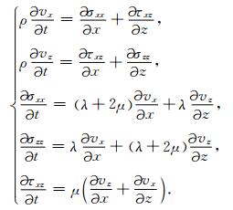
2 波场外推 2.1 波动方程本文采用一阶速度-应力的二维弹性波动方程:
|
(1) |
其中,vx,vz分别为质点的水平分量和垂直分量的振动速度;σxx,σzz分别为水平和垂直方向的正应力,τxz为切应力;ρ为介质的质量密度;λ,μ为介质的拉梅常数;t为时间变量.在波场模拟时,(1)式被离散成空间为高阶(本文采用8阶),时间为二阶精度的交错网格差分[39-41],人工边界采用PML吸收边界条件[42-44]来压制来自边界的反射波.
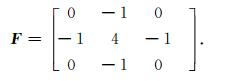
2.2 空间滤波逆时偏移的成像剖面中存在着低频假象[21, 27, 34-35],主要受直达波和震源等的影响.为了高效地去除这部分低频的假象,本文采用空间高通滤波进行去除[5].其滤波系数如下:
|
(2) |
逆时偏移可以分为三个过程:1)震源波场的正向传播,为初值问题;2)检波器波场的逆向传播,将检波器获得的记录按照时间逆序依次插入到对应的记录位置,为边值问题;3)成像条件的应用.本文重点讨论归一化互相关成像条件和激发振幅成像条件,以及改进的稳定激发振幅条件.
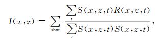
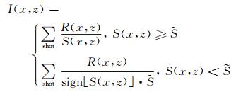
3.1 归一化互相关成像条件归一化互相关成像条件是指通过计算震源波场和接收波场的零延迟互相关,并进行归一化处理[12]:
|
(3) |
其中,S,R分别表示震源波场与检波器波场;

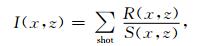
激发振幅成像条件是指通过在震源波场的正传过程,在每个时刻计算出网格点的能量密度,并保存下相应的最大能量密度(见下文)对应的走时和波场值;在检波器波场的逆传过程中,利用保存下的走时提取出相应的检波器波场的波场值,并用保存下的震源波场做归一化,从而得到角度依赖的反射系数剖面,它可以为AVA的分析提供先决条件[33, 45-47].
激发振幅成像条件表达形式为[31]
|
(4) |
其中,S,R分别表示最大能量密度对应的震源波场和提取出的检波器波场;
|
(5) |
其中,
|
(6) |
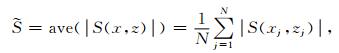
(6)式表示对最大能量密度时刻对应的震源波场值取绝对值后再求平均值,N为二维网格的节点总数.sign[S(x,z)]表示对S(x,z)取符号.相比于弹性波逆时偏移的激发时间成像条件,由于该成像条件用最大能量的震源波场做归一化,自动校正了水平分量在震源两侧的极性反转,且在多炮叠加时避免由于极性反转引起的振幅损失.
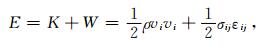
为了获取成像条件所需要的走时和震源波场,在震源波场的正向传播过程中,需要计算能量密度.能量密度[48]的定义如下:
|
(7) |
其中,E,K,W分别表示总能量密度、动能密度和势能密度;σij,εij分别表示应力和应变张量的各个分量,重复的哑元表示求和.
由于本文使用交错网格有限差分,在计算上述能量密度时,需要在时空上进行插值.为了提高计算效率,本文采用线性插值.在震源波场正传的每个时刻,计算各个网格点的能量密度,并与前一时刻保存的该网格点的最大能量密度Ei-1进行比较,若当前时刻的能量密度Ei大于Ei-1,则更新Ei-1、并保存相应的走时Ti-1及波场值R xi-1和R zi-1,直到最大时刻.最终可以获得每个网格相应的最大能量密度对应的走时和震源波场值.当然,在每个时刻进行能量密度的计算,略微增加计算量.
4 数值试验为了验证稳定激发振幅成像条件在弹性波逆时偏移中的有效性,我们分别在倾斜模型、断层模型和Marmousi-ii模型上进行了数值试验.
4.1 倾斜模型倾斜模型(图 1)的网格数为1201×601,网格间距10m,上层的倾角是9°;各层的密度及其纵横波速度详见图 1.检波器间距为10m;采用双边接收观测系统,两侧各布置150道检波器;震源布置在地表,炮间距为200m,共46炮,布置范围为1500~10500m;震源为10Hz的雷克子波的爆炸震源;波场模拟时间间隔为1ms,波场传播至6.0s.

|
图 1 倾斜弹性波模型; 倒三角表示46个炮点位置, 黑色实心三角为第24炮; 虚线为第24炮的偏移孔径 Fig. 1 A elastic wave model with three layer surfaces (includeatiltedsurface); the inverted triangles denote the 46 shots, the filled one corresponding to the 24th shot; dash lines denote the migration aperture of the 24th shot |
图 2为第24炮,采用(7)式计算得到的走时和相应的震源波场值.其中,图 2a为第24炮的偏移孔径内的速度模型,图 2b为计算的走时,图 2(c,d)为最大能量密度时刻的震源波场值;图中虚线表示两个界面的位置.

|
图 2 倾斜模型的第24炮的P波速度模型(a)、最大能量走时等值线(b), x分量的震源波场值(c), 及z分量的震源波场值(d); 虚线表示界面的位置 Fig. 2 P-wave velocity (a), maximum energy traveltime contour (b), source wavefield of x component (c), and source wavefiled of z component (d) of the 24th shot in the model with a tilted surface; dash lines denote the location of the two surfaces in the model |
图 3为对第24炮进行空间高通滤波之前的水平(3a,3c)和垂直(3b,3d)分量的成像剖面.其中,图 3a和3b为归一化互相关成像条件的成像剖面;图 3c和3d为稳定激发振幅成像条件的成像剖面.由于长时程计算,来自边界的虚假反射、以及层间反射波等导致部分虚假反射同相轴(图 3中箭头标注的位置).从图中可以看到,归一化互相关成像条件的成像剖面存在严重的低频假象,如图中椭圆标注范围,垂直分量尤为明显;而激发振幅成像剖面的低频假象比前者弱.从分辨率上看,激发振幅成像条件的分辨率高于归一化互相关成像条件的,尤其表现在垂直分量上,这是因为前者的偏移剖面在量纲上为反射系数,后者的偏移剖面在量纲上为反射系数的平方;从成像能力方面来看,激发振幅成像条件的水平分量优于互相关成像条件的;但是两种成像条件得到的垂直分量的偏移剖面都存在严重的低频假象,这与直达波的切除有着密切的关系;水平分量中存在明显的假象.

|
图 3 倾斜模型的第24炮成像剖面; 归一化互相关成像剖面(a)水平分量; (b)垂直分量; 稳定激发振幅成像剖面:(c)水平分量; (d)垂直分量. Fig. 3 Imaging profiles of the 24th shot in the model with a tilted surface (a) and (b) are the horizontal and vertical component imaging profile from the normalized correlation imaging condition, respectively; (c) and (d) are the horizontal and vertical component imaging profile from the stable excitation amplitude imaging condition, respectively |
图 4是对图 3进行空间高通滤波后的结果.从图中可见,空间高通滤波能高效地去除成像剖面上的低频假象.稳定激发振幅成像条件的水平分量的假象比归一化互相关成像条件的更为严重(如箭头所示),但是前者的分辨率高于后者;并且两种成像条件的垂直分量获得了更加清晰的图像.

图 5为倾斜模型的46炮的叠加结果.从图中可见,由两种成像条件获得的垂直偏移剖面的界面形态比较清晰.由于两端叠加次数仅为1,两端的图像不如中间部分(多次叠加)清楚.对比图 5c和d,不难发现图 5c中的第二个界面比图 5a更加清晰(上述4幅图使用了相同的增益).但是,在水平分量偏移剖面上存在较明显的串扰假象(箭头所指位置)[49].

|
图 5 倾斜模型46炮叠加成像剖面(滤波); 归一化互相关成像剖面 (a)水平分量; (b)垂直分量; 稳定激发振幅成像剖面:(c)水平分量; (d)垂直分量. Fig. 5 Stacked imaging profiles from 46 shots (filtered) in the model with a tilted surface (a) and (b) are the horizontal and vertical component imaging profile from the normalized correlation imaging condition, respectively; (c) and (d) are the horizontal and vertical component imaging profile from the stable excitation amplitude imaging condition, respectively |
为了验证该成像条件在复杂模型中的有效性,我们在断层模型(图 6)上进行了数值试验.该断层模型的网格为1201×601,网格间距为10m;检波器间距为10m;采用双边接收观测系统,两侧各布置200道检波器;震源布置在地表,炮间距为100m,共81炮,布置范围为2000~10000m;震源为10Hz的雷克子波,为爆炸震源;波场模拟时间间隔为1ms;波场传播计算到6.0s.纵、横波速度和密度见图 6所示.

|
图 6 断层模型 Fig. 6 The velocity of the fault model |
图 7为断层模型的81炮叠加结果(未滤波).从图中可见,稳定激发振幅成像条件能够获得与归一化互相关成像条件相当的图像,尤其是断层模型的底部的两个界面,垂直分量能够获得比水平分量更加清晰的图像,且稳定激发振幅成像条件的水平分量的图像比归一化互相关成像条件的清晰.总体上,归一化成像条件得到的偏移剖面低频假象更为严重.同样,在偏移剖面上存在较弱的串扰假象(箭头所指位置)[49].

|
图 7 断层模型的81炮叠加成像剖面(未滤波); 归一化互相关成像剖 (a)水平分量; (b)垂直分量; 稳定激发振幅成像剖面:(c)水平分量; (d)垂直分量. Fig. 7 Stacked imaging profiles from 81 shots (unfiltered) in the fault mode (a) and (b) are the horizontal and vertical component imaging profile from the normalized correlation imaging condition, respectively; (c) and (d) are the horizontal and vertical component imaging profile from the stable excitation amplitude imaging condition, respectively |
为了进一步验证稳定的激发振幅成像条件在非均匀的复杂模型中的有效性,我们将该成像条件应用到石油工业界的标准测试模型--Marmousi-ii弹性波模型中,并与经典的归一化互相关成像条件进行对比研究.其中,图 8是Marmousi-ii的P波速度模型,黑线框内为原始的Marmousi声波模型部分.图 9是Marmousi-ii弹性波模型的构造单元和岩性解释剖面图.相比于原始的Marmousi声波速度模型,Marmousi-ii模型延伸的更长,顶部的水层进一步加厚,并且增加了几个储层和零P波阻抗的砂体(图 9).

|
图 8 Marmousi-ii的P波速度模型 Fig. 8 P-wave velocity of the Marmousi-ii model |

|
图 9 Marmousi-ii模型的构造单元和岩性解释图 Fig. 9 Structural elements and lithologies interpreted map of the Marmousi-ii model |
Marmousi-ii模型的网格点数是13601×2801,受计算条件的限制,我们将其在纵、横向上每间隔5个采样点进行抽稀,最终有2721×561个网格点.稳定的激发振幅成像条件和归一化的互相关成像条件均采用双边接收的观测系统,两侧各布置250道,炮间距为100m,炮点的布置范围为2500~24700m.纵横向网格间距均为10m,时间采样间隔为1ms、震源为10Hz的雷克子波(爆炸震源),震源和检波器均布置在水面,共激发了223炮,波场传播计算到10s.由于逆时偏移算法具有很好的并行性,每个进程可以承担一定炮数的偏移任务,最后再收集进行叠加.为此,该算例使用基于MPI通信的并行程序. Marmousi-ii模型使用16个进程在Dell Precision T5600 WorkStation(linux系统)上进行偏移,偏移结果见图 10.由于两端仅叠加一次,因此两端的图像不如中间清晰.

|
图 10 Marmousi-ii模型的223炮叠加成像剖面(滤波); 归一化互相关成像剖面 (a)水平分量; (b)垂直分量; 稳定激发振幅成像剖面:(c)水平分量; (d)垂直分量. Fig. 10 Stacked imaging profiles of the Marmousi-ii from 223 shots (a) and (b) are the horizontal and vertical component imaging profile from the normalized correlation imaging condition, respectively; (c) and (d) are the horizontal and vertical component imaging profile from the stable excitation amplitude imaging condition, respectively |
从图 10可以看出,总体上,稳定的激发振幅成像条件获得了具有与归一化成像条件相当清晰的偏移剖面,但是后者的低频假象比前者更为严重.两者的水平分量偏移剖面在陡倾构造附近(见断层附近)更加清晰,而垂直分量偏移剖面在低角度构造附近(见左下部分的盐岩上界面)能够获得非常清楚的构造形态,并且四个剖面对(5000m,1700m)处的含气砂岩通道处有很好的响应.
我们将Marmousi-ii模型中最为复杂的部分(水平方向在10000~20000m之间,垂直方向在1000~4000m之间)进行放大比较.从图 11可见,激发振幅成像条件在断层附近能够获得更加清晰的图像,这可能归因于它总是利用波场中信噪比最高的波场信息.

|
图 11 Marmousi-ii模型的部分叠加成像剖面(滤波); 归一化互相关成像剖面 (a)水平分量; (b)垂直分量; 稳定激发振幅成像剖面:(c)水平分量; (d)垂直分量. Fig. 11 Partial stacked imaging profiles of the Marmousi-ii (a) and (b) are the horizontal and vertical component imaging profile from the normalized correlation imaging condition, respectively; (c) and (d) are the horizontal and vertical component imaging profile from the stable excitation amplitude imaging condition, respectively |
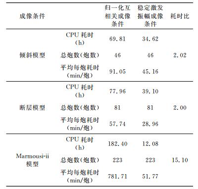
为了对比上述两种成像条件的计算效率,分别统计了上述三个模型的计算时间和对硬盘的需求量(表 1、2).倾斜模型和断层模型在Lenovo Think Centre M8300t(Coreli7,3.40GHz)上测试运行,使用了有限差分串行程序;Marmousi-ii模型在Dell Precision T5600 Work Station(Xeon-8核,2.70GHz)上测试运行,使用了有限差分并行程序.
|
|
表 1 CPU耗时统计 Table 1 The statistic for CPU time consuming |
|
|
表 2 硬盘需求情况统计 Table 2 The statistic for hard disk occupation |
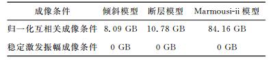
归一化成像条件需要存储波场快照,其硬盘存储空间和I/O吞吐操作是巨大的;而稳定激发振幅成像条件仅需在每个时间步计算能量密度,而其所需要的额外计算量却很小.值得指出的是,由于Marmousi-ii模型的偏移是在工作站Dell Precision T5600进行,使用了最大16个进程,每个进程最多计算14炮,表中的平均每步耗时为总耗时除以14.在单台电脑上运行归一化互相关成像的并行程序,在波场快照的I/O吞吐操作时,各个进程会相互争夺资源,因此其耗时比可能是不客观的,若在多节点的并行机上进行,这个比值可能会降低.受计算条件的限制,对于Marmousi-ii模型,我们每隔2个时间间隔存储波场快照,同样在逆传的过程中每隔2个时刻利用成像条件.即使如此,每炮存储波场信息所需要的硬盘空间为5.26GB,而16个进程需要的硬盘空间多达84.16GB.
4 结论和讨论本文修正了激发振幅成像条件,使其在弹性波逆时偏移中更加稳健.相比于弹性波的归一化互相关成像条件,在成像质量相当的前提下大大节省了存储量,缩短了逆时偏移的总耗时,同时偏移剖面的分辨率较高,低频假象弱,硬盘需求量为零,避免了巨大的I/O吞吐开销,提高了计算效率,这在三维计算(或并行计算)中尤其明显.稳定激发振幅成像利用了波场中信噪比最高的那部分波场(可能是反射波、多次波等)信息,在某些局部区域能够获得相比于归一化互相关成像条件更加清晰的图像.相比于弹性波的激发时间成像条件,稳定激发成像条件使用最大能量的震源波场做归一化,能自动校正水平分量在震源两侧的极性反转,在多炮叠加时避免极性反转引起的振幅损失.归一化互相关成像条件利用了全波场信息,在某些特殊区域(如丘下构造等),它可能获得比稳定激发振幅更加清晰的图像,这些将有待于进一步研究讨论.对于稳定激发振幅成像条件,若走时和震源波场的振幅能通过射线方法(如高斯束[50-51]、波前构建法[52-53])或单频双程波法[54-56]等手段获取,避免了震源波场的正演过程,可能能进一步提高计算效率,但是其成像质量有待于进一步研究讨论.
致谢本文得到中国科学院地质与地球物理研究所滕吉文院士和张忠杰研究员的悉心指导,在此表示衷心的感谢.
| [1] | McMechan G A. Migration by extrapolation of time-dependent boundary values. Geophysical Prospecting , 1983, 31(3): 413-420. DOI:10.1111/gpr.1983.31.issue-3 |
| [2] | Loewnthal D, Mufti I R. Reversed time migration in spatial frequency domain. Geophysics , 1983, 48(5): 627-635. DOI:10.1190/1.1441493 |
| [3] | Whitmore N D. Iterative depth migration by backward time propagation. 53rd Annual International Meeting, SEG, Expanded Abstracts , 1983: 827-830. |
| [4] | McMechan G A, Chang W F. 3D acoustic prestack reverse time migration. Geophysical Prospecting , 1990, 38(7): 737-756. DOI:10.1111/gpr.1990.38.issue-7 |
| [5] | Mulder W A, Plessix R E. A comparison between one-way and two-way wave-equation migration. Geophysics , 2004, 69(6): 1491-1504. DOI:10.1190/1.1836822 |
| [6] | Baysal E, Kosloff D D, Sherwood J W C. Reverse time migration. Geophysics , 1983, 28(11): 1514-1524. |
| [7] | Yoon K, Marfurt K J, Starr W. Challenges in reverse-time migration. SEG Int'1 Exposition and 74th Annual Meeting , 2004. |
| [8] | Zhu J M, Lines L R. Comparison of Kirchhoff and reverse-time migration methods with applications to prestack depth imaging of complex structures. Geophysics , 1998, 63(4): 1166-1176. DOI:10.1190/1.1444416 |
| [9] | Zhang Y, Zhang G Q. One-step extrapolation method for reverse time migration. Geophysics , 2009, 74(4): A29-A33. DOI:10.1190/1.3123476 |
| [10] | Biondi B, Shan G J. Prestack imaging of overturned reflections by reverse time migration. SEG Int'1 Exposition and 72nd Annual Meeting , 2002. |
| [11] | Chattopadhyay S, McMechan G A. Imaging conditions for prestack reverse-time migration. Geophysics , 2008, 73(3): S81-S89. DOI:10.1190/1.2903822 |
| [12] | Claerbout J M. Toward a unified theory of reflector mapping. Geophysics , 1971, 36(3): 467-481. DOI:10.1190/1.1440185 |
| [13] | Kaelin B, Guitton A. Imaging condition for reverse time migration. SEG New Orleans Annual Meeting , 2006. |
| [14] | Yan J, Sava P. Isotropic angle-domain elastic reverse time migration. Geophysics , 2008, 73(6): S229-S239. DOI:10.1190/1.2981241 |
| [15] | Chang W F, McMechan G A. Reverse-time migration of offset vertical seismic profiling data using the excitation-time imaging condition. Geophysics , 1986, 51(1): 67-84. DOI:10.1190/1.1442041 |
| [16] | Alejandro A V, Biondi B. Deconvolution imaging condition for reverse-time migration. Standford Exploration Project , 2002, 112: 83-96. |
| [17] | Costa J C, Silva Neto F A, Alcantara R M, et al. Obliquity-correction imaging condition for reverse time migration. Geophysics , 2009, 74(3): S57-S66. DOI:10.1190/1.3110589 |
| [18] | Yoon K, Marfurt K J. Reverse-time migration using the Poynting vector. Exploration Geophysics , 2006, 37(1): 102-107. DOI:10.1071/EG06102 |
| [19] | Liu F Q, Zhang G Q, Scott A M, et al. Reverse time migration using one-way wavefield imaging condition. 77th Annual Internation Meeting, SEG, Exped Abstracts , 2007, 26(1): 2170-2174. |
| [20] | Baysal E, Kosloff D D, Sherwood J W C. A two-way nonreflecting wave equation. Geophysics , 1984, 49(2): 132-141. DOI:10.1190/1.1441644 |
| [21] | Zhang Y, Sun J. Practical issues of reverse time migration: true amplitude gathers, noise removal harmonic-source encoding. CPS/SEG Beijing 2009 International Geophysical Conference & Exposition , 2009, 27(1): 1-5. |
| [22] | Zhang Y, Xu S, Bleistein N, et al. True-amplitude, angle domain, common-image gathers from one-way wave-equation migrations. Geophysics , 2007, 72(1): S49-S58. DOI:10.1190/1.2399371 |
| [23] | Deng F, McMechan G A. True-amplitude prestack depth migration. Geophysics , 2007, 72(3): S155-S166. DOI:10.1190/1.2714334 |
| [24] | 刘红伟, 李博, 刘洪, 等. 地震叠前逆时偏移高阶有限差分算法及GPU实现. 地球物理学报 , 2010, 53(7): 1725–1733. Liu H W, Li B, Liu H, et al. The algorithm of high order finite differenc pre-stack reverse time migration GPU implementation. Chinese J. Geophys. (in Chinese) , 2010, 53(7): 1725-1733. |
| [25] | 刘红伟, 刘洪, 邹振. 地震叠前逆时偏移中的去噪与存储. 地球物理学报 , 2010, 53(9): 2171–2180. Liu H W, Liu H, Zou Z. The problems of denoise storage in seismic reverse time migration. Chinese J. Geophys. (in Chinese) , 2010, 53(9): 2171-2180. |
| [26] | Loewenthal D, Stoffa P L, Faria E L. Suppressing the unwanted reflections of the full wave equation. Geophysics , 1987, 52(7): 1007-1012. DOI:10.1190/1.1442352 |
| [27] | Fletcher R F, Fowler P, Kitchenside P, et al. Suppressing artifacts in prestack reverse time migration. 75th Annual International Meeting, SEG, Exped Abstracts , 2005, 24(1): 2049-2051. |
| [28] | Feng B, Wang H Z. Reverse time migration with source wavefield reconstruction strategy. J. Geophys. Eng. , 2012, 9(1): 69-74. DOI:10.1088/1742-2132/9/1/008 |
| [29] | Clapp R G. Reverse time migration with random boundaries. 79th Annual International Meeting, SEG Expanded Abstracts , 2009, 28: 2809-2813. |
| [30] | Symes W W. Reverse time migration with optimal checkpointing. Geophysics , 2007, 72(5): SM213-SM221. DOI:10.1190/1.2742686 |
| [31] | Nguyen B D, McMechan G A. Excitation amplitude imaging condition for prestack reverse-time migration. Geophysics , 2013, 78(1): S37-S46. DOI:10.1190/geo2012-0079.1 |
| [32] | Chang W F, McMechan G A. Elastic reverse time migration. Geophysics , 1987, 52(10): 1356-1375. |
| [33] | Schleicher J, Costa J C, Novais A. A comparison of imaging conditions for wave-equation shot-profile migration. Geophysics , 2008, 73(6): S219-S227. DOI:10.1190/1.2976776 |
| [34] | 杨仁虎, 常旭, 刘伊克. 叠前逆时偏移影响因素分析. 地球物理学报 , 2010, 53(8): 1902–1913. Yang R H, Chang X, Liu Y K. The influence factors analyses of imaging precision in pre-stack reverse time migration. Chinese J. Geophys. (in Chinese) , 2010, 53(8): 1902-1913. |
| [35] | Loewenthal D, Hu L Z. Two methods for computing the imaging condition for common shot pre-stack migration. Geophysics , 1991, 56(3): 378-381. DOI:10.1190/1.1443053 |
| [36] | 李文杰, 魏修成, 宁俊瑞, 等. 叠前弹性波逆时深度偏移及波场分离技术探讨. 物探化探计算技术 , 2008, 30(6): 447–456. Li W J, Wei X C, Ning J R, et al. The discussion of reverse time depth migration wavefield separation for pre-stack elastic data. Computing Techniques for Geophysical Geochemical Exploration (in Chinese) , 2008, 30(6): 447-456. |
| [37] | André Bulcao, Djalma Manoel Soares Filho, Webe Joao Mansur. Improved quality of depth images using reverse time migration. 77th Annual International Meeting, SEG Expanded Abstracts, 2007, 26(1): 2407-2411. http://scitation.aip.org/ |
| [38] | Kaelin B, Guitton A. Imaging condition for reverse time migration. In 76th Annual International Meeting Exposition, SEG, Expanded Abstracts , 2006: 2594-2598. |
| [39] | Virieux J. SH-wave propagation in heterogeneous media: velocity-stress finite-difference method. Geophysics , 1984, 49(11): 1933-1942. DOI:10.1190/1.1441605 |
| [40] | Virieux J. P-SV wave propagation in heterogeneous media: velocity-stress finite-difference method. Geophysics , 1986, 51(4): 889-901. DOI:10.1190/1.1442147 |
| [41] | Moczo P, Kristek J, Vavrycuk V, et al. 3D heterogeneous staggered-grid finite-difference modeling of seismic motion with volume harmonic arithmetic averaging of elastic moduli densities. Bull. Seism. Soc. Am. , 2002, 92(8): 3042-3066. DOI:10.1785/0120010167 |
| [42] | Hastings F D, Schneider J B, Broschat S L. Application of the perfectly matched layer (PML) absorbing boundary condition to elastic wave propagation. Journal Acoustical Society of America , 1996, 100(5): 3061-3069. DOI:10.1121/1.417118 |
| [43] | Chew W C, Liu Q H. Using perfectly matched layers for elastodynamics.//Proceedings of the IEEE Antennas and Propagation Society International Symposium. Baltimore, MD, USA: IEEE, 1996, 1: 366-369. |
| [44] | Collino F, Tsogka C. Application of the perfectly matched absorbing layer model to the linear elastodynamic problem in anisotropic heterogeneous media. Geophysics , 2001, 66(1): 294-307. DOI:10.1190/1.1444908 |
| [45] | Hanitzsch C. Comparison of weights in prestack amplitude-preserving Kirchhoff depth migration. Geophysics , 1997, 62(6): 1812-1816. DOI:10.1190/1.1444282 |
| [46] | Baina R, Thierry P, Calandra H, et al. 3D preserved-amplitude prestack depth migration and amplitude versus angle relevance. The Leading Edge , 2002, 21(12): 1237-1241. DOI:10.1190/1.1536141 |
| [47] | 贺振华. 反射地震资料偏移处理与反演方法. 重庆: 重庆大学出版社, 1989 . He Z H. Reflection Seismic Data Migration Processing Inversion (in Chinese). Chongqing: Chongqing University Press, 1989 . |
| [48] | Cerveny V, Molotkov I A, Psencik I. Ray Theory in Seismology. Charles: Charles University Press, 1977 . |
| [49] | Poole T L, Curtis A, Robertsson J O, et al. Deconvolution imaging conditions and cross-talk suppression. Geophysics , 2010, 75(6): W1-W12. DOI:10.1190/1.3493638 |
| [50] | Cerveny V. Ray synthetic seismograms for complex two-dimensional three dimensional structures. J. Geophys. , 1985, 58: 2-26. |
| [51] | Cerveny V. Gaussian beam synthetic seismograms. J. Geophys , 1985, 58: 44-72. |
| [52] | Vinje V, Iversen E, Gjoystdal H. Traveltime apmlitude estimation using wavefront construction. Geophysics , 1993, 58(8): 1157-1166. DOI:10.1190/1.1443499 |
| [53] | Lambará G, Lucio P S, Hanyga A. Two-dimensional multivalued traveltime amplitude maps by uniform sampling of a ray field. Geophys. J. Int. , 1996, 125(2): 584-598. DOI:10.1111/gji.1996.125.issue-2 |
| [54] | Shin C, Min D, Marfurt K J, et al. Traveltime amplitude calculations using the damped wave solution. Geophysics , 2002, 67(5): 1637-1647. DOI:10.1190/1.1512811 |
| [55] | Shin C, Ko S, Kim W, et al. Traveltime calculations from frequency-domain downward-continuation algorithms. Geophysics , 2003, 68(4): 1380-1388. DOI:10.1190/1.1598131 |
| [56] | 秦义龙, 张中杰, ChangsooS, 等. 利用单频双程波动方程计算初至走时及其振幅. 地球物理学报 , 2005, 48(2): 423–428. Qin Y L, Zhang Z J, Changsoo S, et al. First-arrival traveltime and amplitude calculation from monochromatic two-way wave equation in frequency domain. Chinese J. Geophys. (in Chinese) , 2005, 48(2): 423-428. |