 2010, Vol. 53


Double variability space-time of the geomagnetic field is very complex. Continuous monitoring over a long time and maintaining the accuracy of measurements to a standard of quality is the main objective of geomagnetic observatories. At present in the field geomagnetic metrology, precision is 0.1 nT and time is on GPS accuracy. The baseline stability of absolute measurements and quality controls are very important.
The two constituent parts of the geomagnetic field are the main geomagnetic field that is evolving slowly, representing over 90% of the total geomagnetic field, and transient field not exceeding 10% only during periods of extreme agitation field (strong geomagnetic storms).
Part persistence and regular field can be highlighted through mediation for long periods of time. Part transient is represented by deviations from average momentary. It is represented both by the quite and regular changes and by changes shaken and sporadic.
Geomagnetic data analysis can be approached in several ways using different methodologies, e.g., spectral analysis[1~4], wavelet analysis[5, 6], principal component analysis (PCA)[7], etc. Because it is important to know amplitude spectrum and spatial structure of the field in electromagnetic induction studies on the conductivity of the Earth's crust and upper mantle[3], spectral analysis becomes a routine technique in electromagnetic induction studies. Some recent work also showed that spectral analysis is a useful tool in investigating the temporal changes of geomagnetic signals, which may be important for the study on electromagnetic signals possibly associated with earthquakes and volcano eruptions[8~10]. Comparing with spectral analysis, wavelet analysis can provide more information about the frequency characteristics of signal in time domain[5, 6]. While PCA is a powerful method of revealing weak signals from noisy background[7].
This work starts from the general rules for data analysis[1] and applied to geomagnetic data. Based on the above general rules for data analysis, as well as the principles of spectral and wavelet analyses, we develop several programs in MatLab and AutoSignal software (www. mathworks. com) to study geomagnetic field morphology and to determine the spectrum of geomagnetic phenomena in different time intervals. Then we apply the above spectral and wavelet analyses to the geomagnetic data at Kakioka and Vernadsky observatories (http://intermagnet.org). Finally, we discuss the advantages and disadvantages of Fourier Transform and Wavelet Transform.
2 Comparative Analysis of Geomagnetic DataThe link between the phenomena relating to the nature of the causes may be;
(1) Univocal links are directly made between cause-phenomenon and effect-phenomenon. Mathematical relationship for the functional link is;
|
(1) |
(2) Stochastic link, type unknown mathematical function described by

|
(2) |
with reference to the complex phenomena, influenced by many causes.
Dispersion analysis should be used to verify the significance of the group factors (before and after using regression) for calculating and analyzing the results obtained by correlation method (validation model for specific causes). For each pair of registered geophysical parameters, is calculated in the first instance the following indicators (parameters are obtained for n×(n-1)/2 pairs of two-dimensional).
Here's an example of recordings of the geomagnetic field components on period of 24 hours, with a beginning of a geomagnetic storm (Fig. 1).

|
Fig. 1 Geomagnetic field components Hx, Hy, Hz recorded at Surlari Observatory on March 8, 2008. On the abscissa is the number of sampling, the sampling interval being two minutes. |
One way to eliminate the periodic components of the signal is given by the derivation of the signal in relation to the time. In Fig. 2 and Fig. 3 we can see geomagnetic field components derivative depending on the time at the beginning of geomagnetic storm mark with vertical thicken and red line.

|
Fig. 2 Geomagnetic field components Hx, Hy, Hz recorded at Surlari Observatory on March 8, 2008, after signal derivative depending on the time. On the abscissa is the number of sampling, the sampling interval being two minutes |

|
Fig. 3 Derivative of Hy depending on the time (dHy/dt) for three observatories (a) Surlari; (b) Ottawa, (c) Canberra. On the abscissa is the number of sampling, the sampling interval being one minute. The sample 10800 represents the 10800 minutes since March 1, 2008, at 0:00:00 UT until the date of March 8, 2008, at 12:00:00 UT (geomagnetic storm beginning mark with vertical red line). |
Fig. 2 refers to the three orthogonal components of the geomagnetic field recorded at Surlari and Fig. 3 refers to the same component Hy registered in three observatories situated at very different latitudes and longitudes.
Thus we obtain the removal of the periodic components and can see very clearly geomagnetic disturbance.
In the following example can be seen derivatives Hy component of geomagnetic field, depending on time, at 3 observatories located at different coordinates.
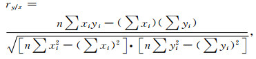
Another way of analyzing the signal is given by the correlation of several sets of data using correlation factor for a two-dimensional series:
|
(3) |
where xi, yi are two series of data; i=l to n; n=number of data in this two series.
Correlation factor is calculated in a mobile window with 10 pairs of values. This mobile window moves on the entire signal step by step. Thus the correlation factor can be calculated for each moment of time ti centered at half window. It can be seen as representing the correlation factor becomes significant change when two time series are causally related. A geomagnetic storm is recorded simultaneously in observatories spread all over the world, but with different amplitudes. The same increase of the variation factor correlation is observed between similar parameters (components of the geomagnetic field) recorded in observatories around the globe during a geomagnetic storm (Fig. 4, Fig. 5).

|
Fig. 4 Correlation factor between two components of the geomagnetic field at beginning of geomagnetic storm, Where: Hnormalized=Hi/Haverage, i=1, …, n |

|
Fig. 5 Correlation factor between normalized total geomagnetic field recorded at Surlari and Canberra Observatories at beginning of geomagnetic storm, where: Hnormalized=Hi/Haverage, i=1, …, n |
The Fast Fourier Transform (FFT) decomposes a time-domain signal (which can be a function of time, spatial coordinates, or any time series abscissa) into complex exponentials (sines and cosines). A Fourier transform offers a complete picture of frequency space, but retains no information as to when in time a signal occurs. Thus a signal should either be wide-sense stationary, with a constant mean and variance across broad time segments, or you must care only qualitatively about whether a certain frequency content signal occurs somewhere in the time range being sampled[2].
The FFT is a fast algorithmic route for producing the Discrete Fourier Transform (DFT).
While the DFT is very simple, it is an order n2 procedure whereas the FFT is an nlog2(n) operation. The difference in processing times is dramatic with large data sets. Fourier decompositions are limited in resolution, as the frequencies at which the sines and cosines are computed are equally spaced and fixed in number. For a data set of n points, there will be n complex frequencies. For real data, the negative frequencies mirror the positive ones, and only the positive frequencies are displayed. Normalized frequencies range from 0, sometimes referred to as DC, to 0.5, the Nyquist frequency, the maximum frequency that can still be detected given the selected sampling rate.
In the following examples spectral analysis data is presented for two geomagnetic observatories INTERMAGNET Program; Kakioka and Vernadsky. You can see the same periodicity at intervals of 8 hours, 12 hours, 24 hours and 28 days[4, 7]. The differences are only in amplitude.
4 Wavelet AnalysisThe Continuous Wavelet Transform (CWT) is used to decompose a signal into wavelets, small oscillations that are highly localized in time. Where as the Fourier transform decomposes a signal into infinitely repeated sines and cosines, effectively losing all time-localization information, the CWT basis functions are scaled and shifted versions of the time-localized mother wavelet. The CWT is used to construct a time-frequency representation of a signal that offers very good time and frequency localization [1, 5, 6].
The CWT is an excellent tool for mapping the changing properties of non-stationary signals. Also is an ideal tool for determining whether or not a signal is stationary. When a signal is judged nonstationary, CWT can be used to identify stationary sections of the data stream. The 1D signal can be analyzed by using wavelet transformation. This can be used to compress the data and to denoise the signal. Wavelet transformation of the 1D signal contains the information regarding the low frequency content of the signal and also the information regarding high frequency content of the signal.
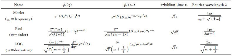
Table 1 show three wavelet basis functions and their properties [5]. H(ω)=Heaviside step function, H(ω)=l if ω > 0, H(ω)=0 otherwise. DOG=derivative of a Gaussian; m=2 is the Marr or Mexican hat wavelet.
|
|
Table 1 Morlet, Paul and derivative of Gaussian wavelet functions[5] |
The wavelet transformation [1, 2] (www.mathworks.com) of the signal use matrix method:
(1) With Haar Transformation
Consider the signal with number of samples N, we form the Haar matrix with size N×N and with the diagonal matrices filled up with the matrix;
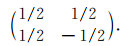
|
(4) |
(2) With Daubechies Transformation
We form the Daubechies Transformation Matrix with diagonal matrices filled up with the matrix;
|
(5) |
Only drawbacks of spectral analysis for geomagnetic data are related to lack the possibility of frequent location in time, amplitude and phase detected in harmonic analysis. Other limitations of harmonic analysis occur if analog or digital signal processing, especially when they are non-stationary phenomena, such as the vast majority of real signals. In this, the harmonic spectrum, calculated using the Fourier transform, is variable in time, but, for convenient length intervals (depending on the frequencies which are used in signal and the rate of change of the spectrum), it can be considered invariant. Plan time-frequency allows us to identify the characteristics of a signal at a time. This is considered a window; moving the signal from the home and? for any position in the timeline window, its content is analyzed, thereby achieving the desired frequency information; a localized spectrum. This information is discrete and finite, so that in plan for -it defines the frequency with time window, a rectangular area, called atom time-frequency.

|
Fig. 6 The spectral analysis of total geomagnetic field recorded at Kakioka Observatory in year 2007×104 Total geomagnetic field at VERNADSKi observatory in period 01 Jan-31 DEC 2007 |

|
Fig. 7 The spectral analysis of total geomagnetic field recorded at Vernadsky Observatory in year 2007 |

|
Fig. 8 Wavelet spectrum for Kakioka and Vernadsky Geomagnetic Observatories during year 2007, from definitive data of INTERMAGNET. Contrasting areas in intensity of red (from light red to dark red) are dependent in function of amplitude spectrum.] |
This atom time-frequency is equivalent to a note signal processing and signal processing operation is to break down their atoms time-frequency. The surface of such atom is 2π, and this causes some problems. For example, we can clarify the spectrum of a signal at a time t0. We instead determine this range for a small range centered at t0. If Δt is low frequency band that we obtain will be higher, thereby decreasing the accuracy of the analysis in frequency. To increase it is necessary to increase the size interval Δt, which results in lower accuracy in time domain analysis. The limit, performing an analysis for interval [0, ∞), we obtain precise information about the spectrum, but the temporal information in the field will no longer be accurate.
The limitations of harmonic analysis occur during processing analog or digital signal, particularly when they are non-stationary phenomena such as the vast majority of real signals.
In the harmonic spectrum, calculated using Fourier transformers, is variable in time, however, for time intervals of convenient length (depending on the frequencies that fall within the signal and speed of change of the spectrum), it-can be considered invariant.
Modeling of these signals can be simultaneously both but considering their properties in time, and those of frequency. The time-frequency allows us to identify the frequency characteristics of signal at a time. For this is considered a mobile window which moves on the signal? starting from t0 to any position on the temporal axis ti, the content is analyzed, there by achieving the desired frequency information: a spectrum of frequencies located.
They are easily visible contrasting areas that align along horizontal lines corresponding to periods of 24 h, 12h and 8 h.
This type of analysis brings us extra information about the relationship spectrum-time. The horizontal axis represents the year 2007 (31, 536, 000 seconds). Vertical axis represents frequency expressed in Hz or period in seconds. We can draw conclusions about the type of magnetic activity associated with time. So on days when contrasting areas are aligned preferentially in the three known periodicity (24 h, 12 h, 8 h) we can say that is quiet days. In the days when contrasting areas not align preferentially on the known periodicity may be interpreted as disturbed days. Between the two wavelet spectra (Kakioka and Vernadsky) are many differences due to local factors;
· Latitude and longitude differences;
· Differences of geological structure involve differences of basement conductivity; in areas with higher conductivity increase in intensity magnetic disturbances, magnetic pre-storms and magnetic storms;
· Characteristics of magnetic events (SI-sudden impulses, SSC-storm sudden commencement, SFE-effect solar flare, B-bays) are dependent of local pattern.

|
Fig. 9 Recordings of geomagnetic storm at many observatories situated at different latitude at May 25~26, 1967 (after Y. Kamide~2006)[11] |
Three sources of low electromagnetic waves are presently known; thunderstorms and related phenomena in the lower atmosphere, tidal wind interaction with ionospheres plasma at dynamic layer heights, solar wind interaction with the magnetosphere.
Sudden geomagnetic variation (SSC, SI, SFE, geomagnetic storms) are relevant through K indices (usually, only for geomagnetic storms calculated for INTERMAGNET observatories). We studied the characteristics of geomagnetic storms and the morphology of geomagnetic field based on the following approaches;
(1) Correlation factor variation, use mobile window, between different components in each observatory, or between some components in different observatories;
(2) Derivative of geomagnetic components versus time;
(3) Frequency analysis (spectral domain);
(4) Wavelet spectrum.
Wavelet series converge uniformly for all continuous functions, while Fourier series do not. Classical wavelets are defined on the real line, while many real world problems are in the finite domain. Periodic and intervallic wavelets have provided part of the solution, but they have also increased the complexity of the algorithm.
Wavelet is a useful tool for analyzing time series for many geophysical parameters with different timescale or changes in variance[5, 6].
Wavelet seem to be very promising in solving many problems for studies pulsations of the geomagnetic field (Pc1-Pc5, Pi1-Pi3) in high frequency with magnetotelluric devices[3] and correlate this data for different observatories. Also, correlate a geomagnetic data with other multi-parametric geophysical data[4, 6~10].
That is why we consider the necessity to stqdy all these types of sources, these reducing from the errors arising from an insufficient knowledge of other sources mechanism.
AcknowledgementsThe results presented in this paper rely on the data collected at Kakioka, Vernadsky, Ottawa and Canberra Geomagnetic Observatories. We thank them for supporting its operation and intermagnet for promoting high standards of magnetic observatory practice (http://intermagnet.org). The manuscript was much improved through the help of the anonymous reviewers and the guest editors.
| [1] | Alfred Mertin.Signal Analysis (Wavelets, Filter Banks, Time-Frequency Transforms and Applications).John Wiley & Sons Ltd., 1999.326 Alfred Mertin.Signal Analysis (Wavelets, Filter Banks, Time-Frequency Transforms and Applications).John Wiley & Sons Ltd., 1999.326 |
| [2] | Catherine Constable.Geomagnetic Temporal Spectrum.In:David Gubbins and Emilio Herrera-Bervera Eds.The Encyclopedia of Geomagnetism and Paleomagnetism.2005 Catherine Constable.Geomagnetic Temporal Spectrum.In:David Gubbins and Emilio Herrera-Bervera Eds.The Encyclopedia of Geomagnetism and Paleomagnetism.2005 |
| [3] | Rokityansky I I.Geoelectromagnetic Investigation of the Earth's Crust and Mantle.Springer-Verlag, New York, 1982.381 Rokityansky I I.Geoelectromagnetic Investigation of the Earth's Crust and Mantle.Springer-Verlag, New York, 1982.381 |
| [4] | Huang Q H, Liu T. Earthquakes and tide response of geoelectric potential field at the Niijima station. Chinese J.Geophy., 2006, 49(6): 1745-1754. |
| [5] | Christopher Torrence, Gilbert P Compo.A practical guide to wavelet analysis.In:Bulletin of the American Meteorological Society-Vol.79, No.1, January 1998, Program in Atmospheric and Oceanic Sciences, University of Colorado, Boulder, Colorado, 1998 Christopher Torrence, Gilbert P Compo.A practical guide to wavelet analysis.In:Bulletin of the American Meteorological Society-Vol.79, No.1, January 1998, Program in Atmospheric and Oceanic Sciences, University of Colorado, Boulder, Colorado, 1998 |
| [6] | George W Pan.Wavelets in Electromagnetics and Device Modeling.John Wiley & Sons, Inc., Hoboken, New Jersey, 2003 George W Pan.Wavelets in Electromagnetics and Device Modeling.John Wiley & Sons, Inc., Hoboken, New Jersey, 2003 |
| [7] | Han P, Huang Q H, Xiu J G. Principal component analysis of geomagnetic diurnal variation associated with earthquakes:case study of the M6.1 Iwate-ken Nairiku Hokubu earthquake. Chinese J.Geophy., 2009, 52(6): 1556-1563. |
| [8] | Huang Q, Ikeya M. Seismic electromagnetic signals (SEMS) explained by a simulation experiment using electromagnetic waves. Phys.Earth Planet.Inter., 1998, 109((3-4)): 107-114. |
| [9] | Du A, Huang Q, Yang S. Epicenter location by abnormal ULF electromagnetic emissions. Geophys.Res.Lett., 2002, 29(10): 1455. DOI:10.1029/2001GL013616 |
| [10] | Nagao T, Enomoto Y, Fujinawa Y, et al. Electromagnetic anomalies associated with 1995 Kobe earthquake. J.Geodyn., 2002, 33((4-5)): 401-411. |
| [11] | Kamide Y.Geomagnetic Storm.Solar Terrestrial Environment Laboratory Nagoya University, Japan.2006 Kamide Y.Geomagnetic Storm.Solar Terrestrial Environment Laboratory Nagoya University, Japan.2006 |