


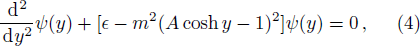
Semi-exact Solutions of Konwent Potential
Cite this Article
Dong Qian, Dong Shi-Shan, Hernández-Márquez Eduardo, Silva-Ortigoza Ramón, Sun Guo-Hua, Dong Shi-Hai. Semi-exact Solutions of Konwent Potential. Communications in Theoretical Physics, 2019, 71(2): 231 
Permissions
Semi-exact Solutions of Konwent Potential
† Corresponding author. E-mail:
Supported by the project under Grant No. 20180677-SIP-IPN, COFAA-IPN, Mexico and partially by the CONACYT project under Grant No. 288856-CB-2016
Abstract
Abstract
In this work we study the quantum system with the symmetric Konwent potential and show how to find its exact solutions. We find that the solutions are given by the confluent Heun function. The eigenvalues have to be calculated numerically because series expansion method does not work due to the variable z ≥ 1. The properties of the wave functions depending on the potential parameter A are illustrated for given potential parameters V0 and a. The wave functions are shrunk towards the origin with the increasing |A|. In particular, the amplitude of wave function of the second excited state moves towards the origin when the positive parameter A decreases. We notice that the energy levels ϵi increase with the increasing potential parameter |A| ≥ 1, but the variation of the energy levels becomes complicated for |A| ∈ (0, 1), which possesses a double well. It is seen that the energy levels ϵi increase with |A| for the parameter interval A ∈ (−1, 0), while they decrease with |A| for the parameter interval A ∈ (0, 1).
1 Introduction
It is well known that the exact solutions of quantum systems play an important role since the early foundation of the quantum mechanics. Generally speaking, two typical examples such as the hydrogen atom and harmonic oscillator have been taken in classical quantum mechanics textbooks.[1–2] Until now, some main methods have been used to solve the quantum soluble systems. First, it is the functional analysis method. That is to say, one solves the second-order differential equation and obtains their solutions[3] given by some well-known special functions. Second, it is called the algebraic method. This method can be realized by studying the Hamiltonian of quantum system and is also related with supersymmetric quantum mechanics (SUSYQM),[4] further closely with the factorization method.[5] Third, it is so-called the exact quantization rule method[6] and proper quantization rule.[7] The latter shows more beauty and symmetry than exact quantization rule. It should be recognized that almost all soluble potentials mentioned above belong to single-well potentials. For example, the classical single-well potential Rosen-Morse potential[8] has been used to treat the vibrations of diatomic molecules such as Na2 and SiC radical[9–10] and to predict successfully the molar enthalpy values, molar entropy values and Gibbs free energies for molecular NO and P2 in a wide temperature range.[11–13] Scattering States of l-wave Schrödinger equation with modified Rosen-Morse potential was also studied.[14] This potential can also be used to construct a double-well potential to treat the vibrations of polyatomic molecules such as the ammonia molecule.[8] The double well potentials[15–23] have been studied for a long time due to their complications and they could be used in the quantum theory of molecules to describe the motion of the particle in the presence of two centers of force, the heterostructures, Bose-Einstein condensates, and superconducting circuits, etc.
Thirty years ago, Konwent proposed an interesting potential[24]

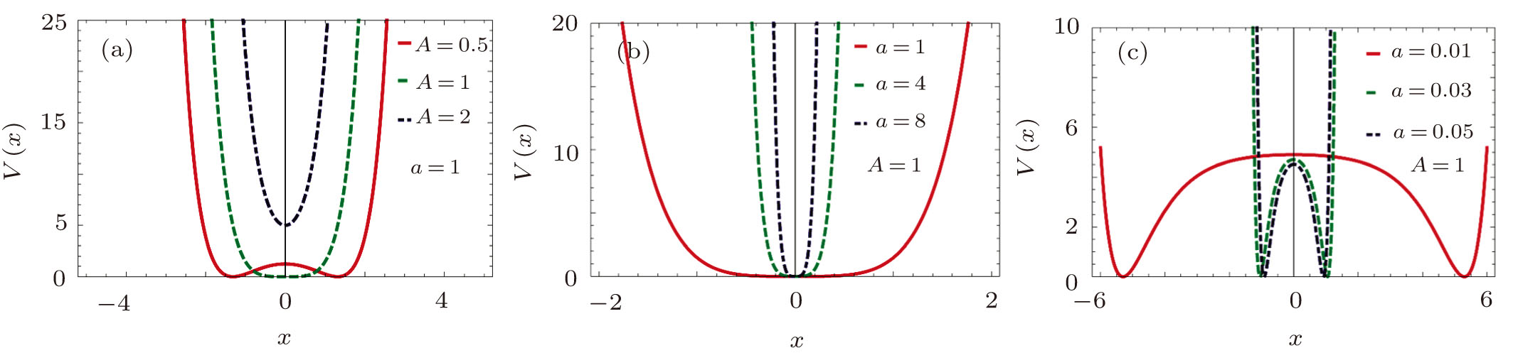 | Fig. 1 (Color online) A plot of potential as function of the variables y and A. |
Through the series expansion around the origin, we have
That is, the solutions cannot be expressed as one of special functions because of three-term recurrence relations. In order to obtain some so-called exact solutions, the authors have to take some constraints on the coefficients in the recurrence relations as shown in Refs. [17, 24]. As shown in recent study of the hyperbolic type potential well,[26–34] we have found that their solutions can be exactly expressed by the confluent Heun function.[29] In this work we attempt to study the solutions of the Konwent potential. We shall find that the solutions can be written as the confluent Heun function but their energy levels have to be calculated numerically since the energy level term is involved in the parameter η of the confluent Heun function Hc (α, β, γ, δ, η z). This constraints us to use the traditional Bathe ansatz method to get the energy levels. It should be pointed out that the Heun function has been studied well, but its main topics are focused in the mathematical area. Only recent connections with the physical problems have been discovered, in particular the quantum systems for those hyperbolic type potential have been studied.[26–34] For this reason, it is not surprising why the authors did not find their solutions related to Heun function.[17,24] The terminology “semi-exact" solutions used in Ref. [27] arise from the fact that the wave functions can be obtained analytically, but the eigenvalues cannot be written out explicitly. The eigenvalues can be calculated by taking the series expansion and then by studying the behaviors of the wave functions at the infinity or by other numerical method.
This paper is organized as follows. In Sec.
2 Semi-exact Solutions
Let us consider the one-dimensional Schrödinger equation,


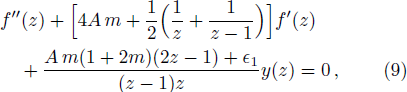
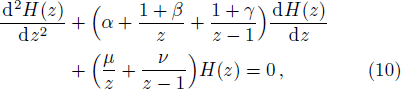
It is found that the parameter η related to energy levels is involved in the confluent Heun function. The wave functions given by this function seem to be analytical, but the key issue is how we first get the energy levels. Otherwise, the solutions become incomplete. Generally, the confluent Heun function can be expressed as a series expansion around the origin
3 Fundamental Properties
In this section we are going to study some basic properties of the wave functions as shown in Figs.
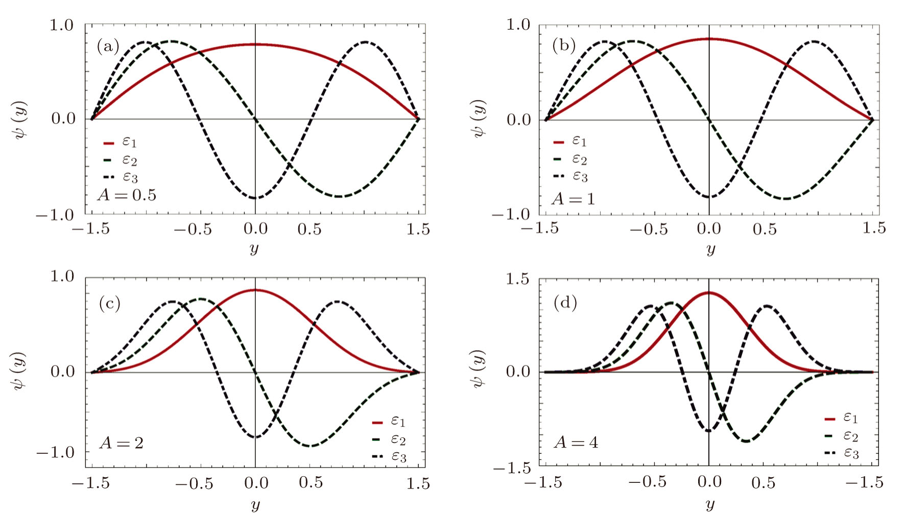 | Fig. 2 (Color online) The characteristics of the wave function as a function of the position y. We take A = 0.5, 1, 2, 4, and V0 = 5, a = 1. |
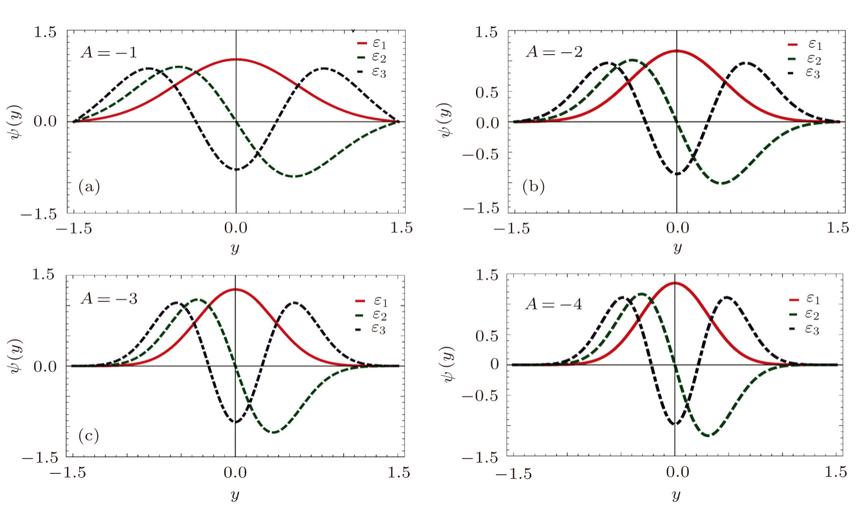 | Fig. 3 (Color online) The characteristics of the wave function as a function of the position y. We take A = −1, −2, −3, −4, and V0 = 5, a = 1. |
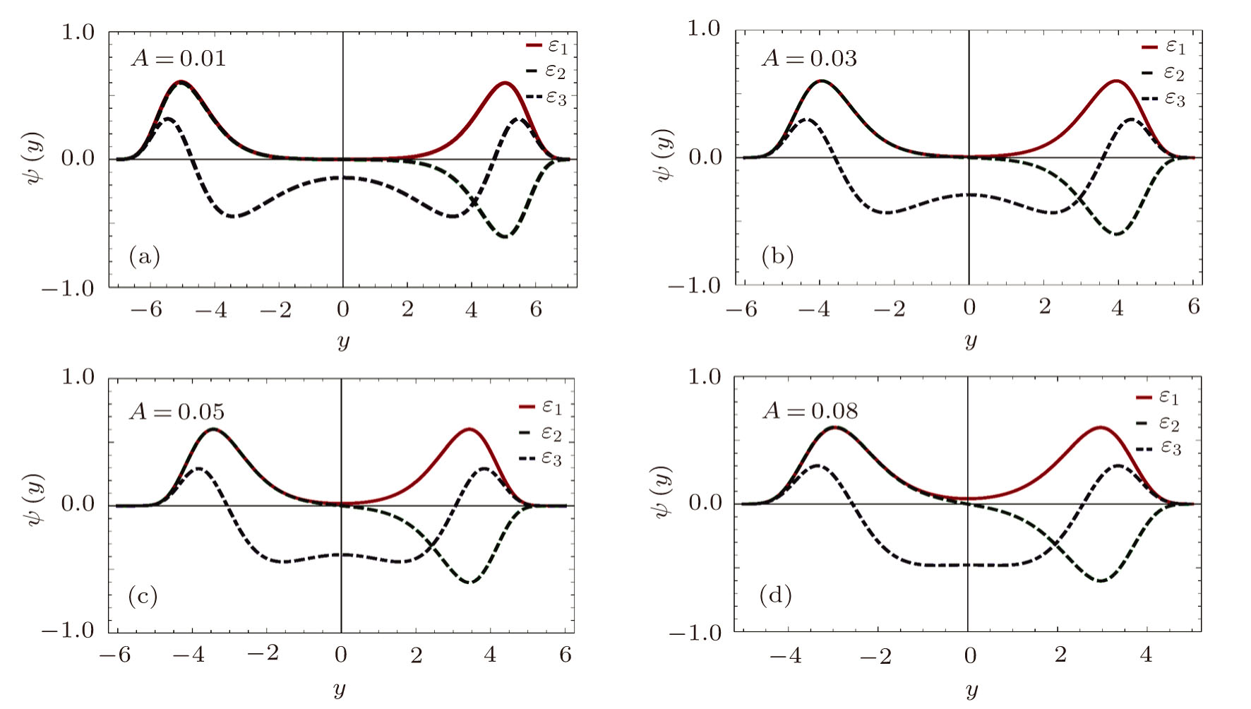 | Fig. 4 (Color online) Same as above case but A = 0.01, 0.03, 0.05, 0.08, and V0 = 5, a = 1. |
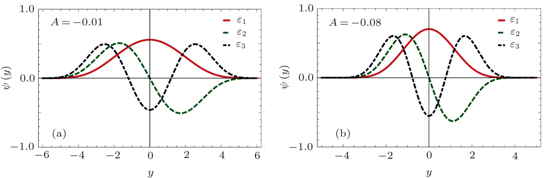
 | Fig. 5 (Color online) Same as above case but A = −0.01, −0.08, and V0 = 5, a = 1. |
| Table 1 Energy levels of the Schrödinger equation with potential (1). . |
We find that the energy levels ϵi increase with the increasing |A| ≥ 1. However, it is seen that the ϵi increase with the parameter |A| for the parameter interval A ∈ (−1, 0), while they decrease with |A| for the parameter interval A ∈ (0, 1). As we know, the wave functions are given by ψ(z) = em A(2z − 1) Hc(α, β, γ, δ, η; z). Generally speaking, the wave functions require ψ(z) → 0 when z → ∞, i.e., x → ∞. Unfortunately, the present study is unlike our previous study,[26–27] in which z → 1 when x goes to infinity. The energy spectra can be calculated by taking the limit z → 1 after the series expansion. In addition, on the contrary to the case discussed by Konwent,[24] in which he supposed the A is taken positive, we also notice that the A can also be taken negative. In this case, the minimum value of single well will be lifted relatively. The wave functions relevant for the positive and negative A are plotted in Figs.
We find that the wave functions are shrunk towards the origin with the increasing |A|. This makes the amplitude of the wave functions be increasing. For the small positive and negative A, however, the change of the wave functions is very sensitive to the parameter A, the wave functions are also shrunk towards the origin with the increasing |A| as shown in Figs.
4 Conclusions
In this work we have studied the quantum system with the symmetric Konwent potential and shown how its exact solutions are found by transforming the original differential equation into a confluent type Heun differential equation. It is found that the solutions can be expressed by the confluent Heun function Hc (α, β, γ, δ, η; z), in which the energy levels are involved inside the parameter η. This makes us calculate the eigenvalues numerically in another way. The properties of the wave functions depending on the parameter A are illustrated graphically for given potential parameters V0 and a. We have also noticed that the energy levels ϵi increase with the increasing potential parameter |A| ≥ 1 corresponding to a single well potential. Finally, we see that the ϵi increase with the increasing |A| for the parameter interval 0 > A > − 1, while they decrease with the increasing |A| for the parameter interval 0 < A < 1.
Reference
| [1] | |
| [2] | |
| [3] | |
| [4] | |
| [5] | |
| [6] | |
| [7] | |
| [8] | |
| [9] | |
| [10] | |
| [11] | |
| [12] | |
| [13] | |
| [14] | |
| [15] | |
| [16] | |
| [17] | |
| [18] | |
| [19] | |
| [20] | |
| [21] | |
| [22] | |
| [23] | |
| [24] | |
| [25] | |
| [26] | |
| [27] | |
| [28] | |
| [29] | |
| [30] | |
| [31] | |
| [32] | |
| [33] | |
| [34] |