


Solitary Wave Solutions of KP equation, Cylindrical KP Equation and Spherical KP Equation
Cite this Article
Li Xiang-Zheng, Zhang Jin-Liang, Wang Ming-Liang. Solitary Wave Solutions of KP equation, Cylindrical KP Equation and Spherical KP Equation. Communications in Theoretical Physics, 2017, 67(2): 207 
Permissions
Solitary Wave Solutions of KP equation, Cylindrical KP Equation and Spherical KP Equation
† Corresponding author. E-mail:
Supported by the National Natural Science Foundation of China under Grant No. 11301153 and the Doctoral Foundation of Henan University of Science and Technology under Grant No. 09001562, and the Science and Technology Innovation Platform of Henan University of Science and Technology under Grant No. 2015XPT001
Abstract
Abstract
Three (2+1)-dimensional equations–KP equation, cylindrical KP equation and spherical KP equation, have been reduced to the same KdV equation by different transformation of variables respectively. Since the single solitary wave solution and 2-solitary wave solution of the KdV equation have been known already, substituting the solutions of the KdV equation into the corresponding transformation of variables respectively, the single and 2-solitary wave solutions of the three (2+1)-dimensional equations can be obtained successfully.
Keyword:2-Solitary wave solution;KP equation;cylindrical KP equation;spherical KP equation;transformation of variables
1 Introduction
Many famous nonlinear evolution equations such as Korteweg-de Vries (KdV), Modified KdV (mKdV), Kadomstev–Perviashvili (KP), Coupled KP and Zakharov–Kuznetsov (ZK) have been obtained in nonlinear propagation of dust-acoustic wave, especially, the dust-acoustic solitary wave (DASW) in space and laboratory plasma.[1] It is known that the transverse perturbations always exist in the higher-dimensional system. Anisotropy is introduced into the system and the wave structure and stability are modified by the transverse perturbation. Recent theoretical studies for ion-acoustic/dust-acoustic waves show that the properties of solitary waves in bounded nonplanar cylindrical/spherical geometry differ from that in unbounded planar geometry. A dissipative cylindrical/spherical KdV is obtained by using the standard reductive perturbation method in Ref. [2]. The cylindrical KP equation (CKP) has been introduced by Johnson[3–4] to describe surface wave in a shallow incompressible fluid. A spherical KP (SKP) equation is obtained by using the standard reductive perturbation method.[5]
We consider the classical KP equation in the form
The cylindrical KP equation (CKP)
We also consider the classical spherical KP equation (SKP) in the form
The KdV equation has been researched by many authors. The multi-soliton solutions of the KdV equation with general variable coefficients have been completely obtained by homogeneous balance principle.[9–10] Some solutions, which possess movable singular points while their energies are only redistributed without dissipation, of KdV equation have been obtained through the modified bilinear Bäcklund transformation.[11] An n-soliton solution with the bell shape has been obtained in Ref. [12], whose stationary height is an arbitrary constant c. The rational solutions, solitary wave solutions, triangular periodic solutions, Jacobi periodic wave solutions and implicit function solutions of KdV equation have been constructed by means of an extended algebraic method.[13] If a transformation of variables between the KdV equation and other equation can be constructed, the results of KdV equation above can be used directly.
In the present paper we aim to find solitary wave solutions of KP Eq. (
2 Reduction of KP, CKP and SKP
2.1 Reduction of KP4 ) into Eq. (1 ), yields an equation as follows
7 ) the expression (4) becomes
In Eq. (
Setting the coefficients of wξ and wξξ to zero, yields
The system (6) admits the following solution:
And after integrating (5) with respect to ξ once and taking the constant of integration to zero, Eq. (
From the discussion above, we come to the conclusion that the KP Eq. (
2.2 Reduction of CKP10 ) into Eq. (2 ), yields an equation as follows
In Eq. (
Setting the coefficients of wξ and wξξ to zero, yields
The system (12) admits a solution:
Using Eq. (
And after integrating (11) with respect to ξ once and taking the constant of integration to zero, Eq. (
From the discussion above, we come to the conclusion that the CKP Eq. (
2.3 Reduction of SKP15 ) into Eq. (3 ), yields an equation as follows
18 ) the expression (15) becomes
16 ) once, taking the constant of integration to zero, Eq. (16 ) becomes the classical KdV Eq. (9 ).
In Eq. (
Setting the coefficients of wξ and wξξ to zero, yields
The system (17) admits a solution:
From the discussion above, we come to the conclusion that the SKP Eq. (
3 Solitary Wave Solutions of KP, CKP and SKP9 ) also has 2-soliton solution
In previous section, the KP Eq. (
3.1 Solitary Wave Solutions of KP
Substituting Eq. (
Substituting Eq. (

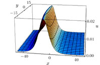
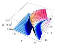
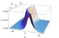
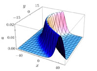
3.2 Solitary Wave Solutions of CKP1 –4 with k = 0.2, x0 = 3, α = 1.
Substituting Eq. (
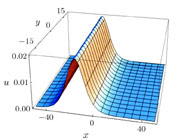 | Fig. 1 Plots of solution (24) with t = 0. |
 | Fig. 2 Plots of solution (24) with t = 0.1. |
 | Fig. 3 Plots of solution (24) with t = 0.5. |
 | Fig. 4 Plots of solution (24) with t = 1. |
Substituting Eq. (
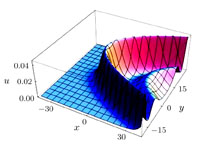
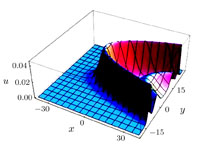
The solution (25) is shown in Figs.
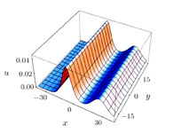 | Fig. 5 Plots of solution (25) with t = 0. |
 | Fig. 6 Plots of solution (25) with t = 0.5. |
 | Fig. 7 Plots of solution (25) with t = 1. |
 | Fig. 8 Plots of solution (25) with t = 2. |
3.3 Solitary Wave Solutions of SKP
Substituting Eq. (
Substituting Eq. (

4 Conclusion
In this paper, by making corresponding transformation of variables, the KP equation, cylindrical KP equation and spherical KP equation are all reduced to the same classical KdV equation, which can be solved by using homogeneous balance method[9–10] to obtain single solitary wave solution and 2-soliton solution. Substitutiong the solitary solutions of the KdV equation into the corresponding transformation of variables, we have the solitary wave solutions of the KP equation, cylindrical KP equation and spherical KP equation, respectively. It is interesting to research CKP equation and SKP equation but avoid the singularity point analysis when t = 0. The analysis in the present paper may be extended to other works to make further progress.
Reference
| [1] | |
| [2] | |
| [3] | |
| [4] | |
| [5] | |
| [6] | |
| [7] | |
| [8] | |
| [9] | |
| [10] | |
| [11] | |
| [12] | |
| [13] |