1 Introduction

Landslides are a common type of geohazard observed in mountainous areas all around the world, typically bringing serious damages in their aftermath. When a landslide occurs around a water body, the impulsive waves generated by the rushed mass may result in even greater consequences than the landslide itself (Xiao et al., 2015). This is especially true in confined areas (Panizzo et al., 2005), such as channelized rivers or reservoirs. Often considered the 'generator' of waves, landslides have various types and may be either rigid or deformable. Deformable landslides usually occur in the deep-valleyed bank, flowing to the river as a type of viscous flow. During the sliding process, the morphological and kinematic characteristics of the landslide change significantly.

One example is the LGW event that occurred in Lituya Bay, Alaska in 1958 (Fritz, 2001). This event involved a rockslide with a volume of 30 million m³ that plugged into the water along a 40˚ slope, with velocity estimated to be around 110 m s⁻¹ running up to the opposite bank with a height of 524 m, thereby destroying all trees and causing two deaths and two boats to go missing (Slingerland and Voight, 1979). The subsequent experiment conducted by Fritz (2001) revealed that before the slide came into contact with the water, the thickness of the front mass increased by about 40%, while the length of the slide decreased from 970 m to 748 m, thus showing significant deformation features. During the earthquake-induced Maruyama landslide in Japan in 1972, it was reported that the slide thickness dramatically decreased from 100 m to 30 m, revealing a stretched morphology during the long-distance movement (Miyamoto, 2010). Another event occurred in the Three Gorges Reservoir on November 23, 2008, during which the Gongjiafang landslide plugged into the Yangtze River, resulting in waves with a maximum amplitude of 31.8 m (Huang et al., 2012). The rockslide decomposed into debris with a volume of 0.5 million m³, showing evident flow and deformable behavior while traveling (Huang and Dai, 2014).

Due to the strong solid-fluid interaction and energy exchange, LGWs are considered hazardous events in near-fields, greatly threatening navigation safety and the safety of the people and infrastructure surrounding the affected regions. An effective way to mitigate such a hazard is to predict the near-field characteristics of the impulsive waves, such as the wave amplitude, run-up to the opposite bank, and so on (Noda, 1970; Frtiz et al., 2003; Heller et al., 2009; Heller and Hager, 2010; McFall and Fritz, 2016; Chen et al., 2020; Romano et al., 2020). The predicted wave features can then be used as the essential data to zone risk maps and issue early warnings, among other measures (McAdoo and Watts, 2004; Masson et al., 2006; Puddasaini, 2014).

Many studies have reported that wave characteristics are closely related to the shape variation and dynamics of landslides during the movement. Experiments conducted by Fritz et al. (2003) revealed that a landslide composed by particle materials could result in different waves compared with that comprising a rigid body due to its strong deformation. The rigid slide-derived equations may overestimate the wave amplitude of LGW for deformable landslide cases by failing to consider the morphological changes involved (Yavari-Ramshe and Ataie-Ashtiani, 2017). The wave difference between a deformable and rigid landslide becomes even more obvious if larger deformations and longer migration distances are involved (Løvholt et al., 2015). In particular, the flow state of a landslide at the time of water-slide contact and the subsequent interactions are key factors in determining the near-field characteristics (Heller, 2007; Heller and Hager, 2010, 2014). Therefore, special attention should be paid to the type of deformable landslides in near-field wave characteristics evaluation.

To date, the methods to study a landslide's near-field characteristics and dispersion can be categorized into three groups, empirical or analytical methods (Kennard, 1949; Haugen et al., 2005; Di Risio and Sammarco, 2008), physical experiment-based methods (Noda, 1970; Fritz, 2001; Di Risio et al., 2009; Heller and Hager, 2010; Wang et al., 2017), and numerical methods (Quecedo et al., 2004; Dai et al., 2014; Wang et al., 2016c; Ruffini et al., 2019; Attili et al., 2021). Empirical methods are capable of quick prediction of wave characteristics by using simplified parameters. However, only a limited understanding of the complicated mechanisms can be obtained using these methods because the motion process and deformation characteristics of landslides are seldom considered. In terms of physical experiment-based methods, its advantage is that the full process of landslide-water interaction, wave generation, propagation, and run-up can be directly observed. In addition, more reliable results can be obtained by applying proportion rules. Nevertheless, the preparation for and conduct of a specific experiment is time-consuming and usually costly. In addition, the scale effects of the physical model may affect the results because it is nearly impossible to reproduce a field case in the lab with the same scale and settings. As an alternative, numerical simulation is a widely accepted method of studying LGW by taking advantage of accurate and visualized presentation of landslide dynamics and its interaction with water.

In the past few decades, the grid-based Euler method has played a leading role in this research field, including finite difference method (Fine et al., 2005; Horrillo et al., 2013), finite element method (Quecedo et al., 2004; Pasenow et al., 2008; Cecioni and Bellotti, 2010), finite volume method (Bosa and Petti, 2011; Ma et al., 2012; Macías et al., 2015), and boundary element method (Harbitz et al., 2014; Schaub et al., 2016). However, for LGWs dominated by free surface flows, the grid-based methods are restricted from capturing the high-degree nonlinearity and discontinuity on the fixed Euler mesh (Cleary and Prakash, 2004), such as the large displaced slide body, the splashing and fragmentation of water in the wave generation, and so on. To overcome such limitations, some meshless numerical methods have been proposed, resulting in their considerable progress and extensive utilization in fluid dynamics simulation in recent years (Cleary and Prakash, 2004; Hori et al., 2011).

One example is the smooth particle hydrodynamics (SPH) method, which is highly effective in simulating free surface fluid dynamics, such as the LGW, due to its meshless nature (Ataie-Ashtiani and Shobeyri, 2008; Qiu, 2008; Wang et al., 2016a). Previous studies have considered landslides as rigid blocks with simple geometry. Some applications also predefined the rigid landslide movement, which can lead to the absence of a true landslide-water interaction (Viroulet et al., 2013; Shi et al., 2015; Wang et al., 2016b). The above treatment may be able to derive reasonable or right results for relatively rigid landslides, which are less deformed during the sliding or interaction process. However, this method is not suitable for dealing with deformable landslides, especially for those consisting of cracked rock boulders or debris.

The proper reproduction of deformable landslide dynamics is crucial in the accurate prediction of the near-field waves. Generally, the movement of the deformable landslide can be treated as a kind of viscous granular flow; thus, its simulation involves multiphase modeling. In particular, the water is described by Newtonian flow, while the flowing behavior of the landslide can be generalized as a kind of nonNewtonian fluid by applying proper rheological model. To date, the most commonly used nonNewtonian models are the Bingham model (Bingham, 1922; Capone et al., 2010; Pastor et al., 2014), the bilinear model (Hosseini et al., 2007), the Cross model (Shao and Lo, 2003), the viscosity regularization model (Minatti and Paris, 2015), and the Herschel-Bulkley-Papanastasiou model (Papanastasiou, 1987; Mitsoulis, 2007), among others. In these models, viscosity is defined as a function of magnitude of the shear rate tensor. These models also have slight differences in terms of the application of different parameters and the way they handle the yielding criterion.

In this study, the HBP model was employed to describe the rheological behaviors of deformable landslides under the SPH framework. Two cases, namely, the simplified Lituya LGW experiment and the practical Gongjiafang LGW, were used to validate the method and demonstrate the performance of the proposed model. Finally, the effect of control parameters of the HBP model on the landslide dynamics and wave features are discussed.

2 Fundamentals of the SPH Method

The SPH method is based on interpolation theory and is considered a 'truly' meshless method for obtaining approximated numerical solutions for differential equations (Monaghan, 1994; Hosseini et al., 2007; Liu and Liu, 2010). Unlike grid-based methods, in the SPH method, the computational domain of a defined problem is discretized by a set of particles associated with field variable information, such as density, pressure, and temperature. Furthermore, unlike in the finite element and finite volume methods, connectivity data are not required. This unique meshless feature of the SPH method makes it highly useful when dealing with complex flows exhibiting large deformations and free surface. The key technique of the SPH method is approximation, particularly kernel and particle approximation.

2.1 Approximation Techniques

In the SPH method, any function can be expressed by its values at a set of points over the region of interest by using a kernel function with an integral form. This is the kernel approximation technique with the following general form:

$ \left\langle {f(\boldsymbol x)} \right\rangle = \int_\Omega {f(\boldsymbol x')} W\left({\boldsymbol x - \boldsymbol x', h} \right){\text{d}}x', $

(1)

where the function f (x) represents either scalar or tensor quantity and is closely related to the point position x, and x is the vector (x, y, z) in three dimensions. The volume of the integral including x is Ω. In addition, W(x − x', h) is the smoothing/kernel function with a finite radius h defining the support area. The kernel function W is usually an even function and must fulfill some conditions, such as the unity condition, the delta function condition, and the compact condition. In this study, we employed the quintic Wendland function:

$ W(\boldsymbol x - \boldsymbol x', h) = {\alpha _D}{\left({1 - \frac{q}{2}} \right)^4}(2q + 1), {\text{ }}0 \leqslant q \leqslant 2, $

(2)

where $q = \frac{{\left| {\boldsymbol x - \boldsymbol x'} \right|}}{h}$ is the relative distance between two points, and α_D is $ \frac{7}{{4{{\rm{ \mathsf{ π} }}}{h^2}}} $ and $\frac{{21}}{{16{{\rm{ \mathsf{ π} }}}{h^3}}}$ are for the two- and three-dimensional problems, respectively.

Similarly, the kernel approximation of the derivative of a spatial function ∇·f (x) can be simply derived by substituting f (x) with ∇·f (x) in Eq. (1), thus yielding:

$ \left\langle {\nabla \cdot f(\boldsymbol x)} \right\rangle = \int_\Omega {\left[ {\nabla \cdot f(\boldsymbol x')} \right]} \cdot W(\boldsymbol x - \boldsymbol x', h){\text{d}}\boldsymbol x' . $

(3)

By applying the expanding form of [∇·f (x')]·W(x − x', h) illustrated in Eq. (4) and by using the divergence theorem, we can obtain the kernel approximation for a function derivative shown in Eq. (5):

$ \begin{aligned} & {\left[\nabla \cdot f\left(\boldsymbol{x}^{\prime}\right)\right] \cdot W\left(\boldsymbol{x}-\boldsymbol{x}^{\prime}, h\right)=} \\ & \qquad \nabla \cdot\left[f\left(\boldsymbol{x}^{\prime}\right) W\left(\boldsymbol{x}-\boldsymbol{x}^{\prime}, h\right)\right]-f\left(\boldsymbol{x}^{\prime}\right) \nabla \cdot\left[W\left(\boldsymbol{x}-\boldsymbol{x}^{\prime}, h\right)\right], \end{aligned} $

(4)

$ \left\langle {\nabla \cdot f(x)} \right\rangle = - \int_\Omega {f(\boldsymbol x')} \cdot \nabla W(\boldsymbol x - \boldsymbol x', h){\text{d}}\boldsymbol x' . $

(5)

As can be clearly seen, in Eq. (5), the process of obtaining the differential of a function is transformed into solving the differential of the kernel function. The second technique of the SPH method is the particle approximation, which presents the domain of interest by a set of particles. In this step, the domain Ω is filled with ordered particles, and the value of the field function f (x) at a specific particle i is evaluated by summation of the values of the surrounding particles j. With particle approximation, the continuous form of kernel approximation expressed in Eqs. (1) and (5) can be rewritten in discretized form as

$ \left\langle {f({\boldsymbol x_i})} \right\rangle = \sum\limits_{j = 1}^N {\frac{{{m_j}}}{{{\rho _j}}}} f({\boldsymbol x_j})W({\boldsymbol x_i} - {\boldsymbol x_j}, h), $

(6)

$ \left\langle {\nabla \cdot f({\boldsymbol x_i})} \right\rangle = - \sum\limits_{j = 1}^N {\frac{{{m_j}}}{{{\rho _j}}}} f({\boldsymbol x_j}) \cdot \nabla W({\boldsymbol x_i} - {\boldsymbol x_j}, h), $

(7)

where N is the total number of surrounding particles, ∇W is evaluated at particle j, and m_j and ρ_j are the mass and density of particle j, respectively. The use of particle summations to approximate integrals is the core technique that facilitates the easy application of the SPH method for programming using a background mesh.

2.2 SPH Formulations for Modeling Hydrodynamics

The general equations governing fluid dynamics are the Navier-Stokes (N-S) equations derived using the principles of mass and momentum conservation. The original form of the N-S equations is shown in Eq. (8). Using the previously introduced SPH approximation techniques, it is possible to translate the original partial differential equations into the SPH notation as shown in Eq. (9):

$ \left\{ {\begin{array}{*{20}{l}} {\frac{{{\text{d}}\rho }}{{{\text{d}}t}} = - \rho \frac{{\partial {\boldsymbol v^\alpha }}}{{\partial {\boldsymbol x^\alpha }}}} \\ {\frac{{{\text{d}}{v^\alpha }}}{{{\text{d}}t}} = \frac{1}{\rho }\frac{{\partial {\boldsymbol \sigma ^{\alpha \beta }}}}{{\partial {\boldsymbol x^\beta }}} + {\boldsymbol g^\alpha }} \end{array}} \right., $

(8)

$ \left\{ {\begin{array}{*{20}{l}} {\frac{{{\text{d}}{\rho _i}}}{{{\text{d}}t}} = \sum\limits_{j = 1}^N {{m_j}\left({\boldsymbol v_i^\alpha - \boldsymbol v_j^\alpha } \right)\frac{{\partial {W_{ij}}}}{{\partial x_i^\alpha }}} } \\ {\frac{{{\text{d}}\boldsymbol v_i^\alpha }}{{{\text{d}}t}} = - \sum\limits_{j = 1}^N {{m_j}\left({\frac{{\boldsymbol \sigma _i^{\alpha \beta }}}{{\rho _i^2}} + \frac{{\boldsymbol \sigma _j^{\alpha \beta }}}{{\rho _j^2}}} \right)\frac{{\partial {W_{ij}}}}{{\partial \boldsymbol x_i^\beta }}} + \boldsymbol g_i^\alpha } \end{array}} \right., $

(9)

where v^α is the velocity vector, σ^αβ is the total stress tensor, g^α is the gravity vector taken as (0, 0, −9.81) m s⁻², and $ \frac{{\partial {W_{ij}}}}{{\partial \boldsymbol x_i^\alpha }} = \frac{{\partial W\left({\boldsymbol x_i^\alpha - \boldsymbol x_j^\alpha, h} \right)}}{{\partial \boldsymbol x_i^\alpha }} $ is the gradient of the kernel evaluated at particle i. An artificial viscosity Π_ij is typically added to the right-hand side of the momentum equation to convert the kinetic energy into heat (Monaghan, 1992). This treatment helps avoid numerical oscillations and resists penetration between particles. The typical form for Π_ij is expressed as

$ {\Pi _{ij}} = \left\{ {\begin{array}{*{20}{l}} {\frac{{ - k{{\bar c}_{ij}}{\xi _{ij}}}}{{{{\bar \rho }_{ij}}}}, {\text{ }}(\boldsymbol v_i^\alpha - \boldsymbol v_j^\alpha)(\boldsymbol x_i^\alpha - \boldsymbol x_j^\alpha) < 0} \\ {0, {\text{ }}(\boldsymbol v_i^\alpha - \boldsymbol v_j^\alpha)(\boldsymbol x_i^\alpha - \boldsymbol x_j^\alpha) > 0} \end{array}} \right., $

(10)

$ {\xi _{ij}} = \frac{{h(\boldsymbol v_i^\alpha - \boldsymbol v_j^\alpha)(\boldsymbol x_i^\alpha - \boldsymbol x_j^\alpha)}}{{{{\left| {\boldsymbol x_i^\alpha - \boldsymbol x_j^\alpha } \right|}^2} + 0.01{h^2}}}, $

(11)

where k is a constant parameter that should be adjusted to introduce proper dissipation. In addition, $ {\bar c_{ij}} = \frac{{{c_i} + {c_j}}}{2} $ is the mean speed of sound, and $ {\bar \rho _{ij}} = \frac{{{\rho _i} + {\rho _j}}}{2} $ is the mean density.

3 Rheological Investigation of Granular Material Behavior and Modeling Platform 3.1 General Relationships

The total stress tensor σ^αβ in Eq. (9) consists of two portions shown in Eq. (12):

$ {\boldsymbol \sigma ^{\alpha \beta }} = - p{\boldsymbol \delta ^{\alpha \beta }} + {\boldsymbol \tau ^{\alpha \beta }}, {\text{ }}\left({{\boldsymbol \delta ^{\alpha \beta }} = \left\{ {\begin{array}{*{20}{c}} {\begin{array}{*{20}{c}} 1&{\alpha = \beta } \end{array}} \\ {\begin{array}{*{20}{c}} 0&{\alpha \ne \beta } \end{array}} \end{array}} \right.} \right) . $

(12)

The first portion is the isotropic pressure p, which is calculated by the local densities by the Equation of State (EoS):

$ p = B\left[ {{{\left({\frac{\rho }{{{\rho _0}}}} \right)}^\gamma } - 1} \right], $

(13)

where constant $ B = \frac{{c_0^2{\rho _0}}}{\gamma } $, ρ₀ is the reference density, c₀ is the speed of sound at reference density calculated by B = $ \beta \sqrt {g{h_{\max }}} $. β is a constant, and γ is a dimensionless parameter. The remaining portion of the total stress tensor equation is the viscous shear stress τ^αβ. Using the proper constitutive model to describe the shear stress τ^αβ, one can model the dynamics of both Newtonian and nonNewtonian fluids by solving Eq. (9). The general form of the shear stress tensor is given by

$ {\tau ^{\alpha \beta }}{\text{ = }}\mu {\boldsymbol D^{\alpha \beta }}, $

(14)

where μ is the viscosity of the fluid, and D^αβ is the shear strain rate tensor equals $ \frac{1}{2}\left({\frac{{\partial {\boldsymbol v^\alpha }}}{{\partial {\boldsymbol x^\beta }}} + \frac{{\partial {\boldsymbol v^\beta }}}{{\partial {\boldsymbol x^\alpha }}}} \right) $. Assuming the velocity vector v^α = (u, v, w)^T and position vector x^α = (x, y, z)^T, the shear strain rate tensor can be rewritten in the expanded form as

$ {\boldsymbol D^{\alpha \beta }} = \left({\begin{array}{*{20}{c}} {\frac{{\partial u}}{{\partial x}}}&{\frac{1}{2}\left({\frac{{\partial u}}{{\partial y}} + \frac{{\partial v}}{{\partial x}}} \right)}&{\frac{1}{2}\left({\frac{{\partial u}}{{\partial z}} + \frac{{\partial w}}{{\partial x}}} \right)} \\ {\frac{1}{2}\left({\frac{{\partial v}}{{\partial x}} + \frac{{\partial u}}{{\partial y}}} \right)}&{\frac{{\partial v}}{{\partial y}}}&{\frac{1}{2}\left({\frac{{\partial v}}{{\partial z}} + \frac{{\partial w}}{{\partial y}}} \right)} \\ {\frac{1}{2}\left({\frac{{\partial w}}{{\partial x}} + \frac{{\partial u}}{{\partial z}}} \right)}&{\frac{1}{2}\left({\frac{{\partial w}}{{\partial y}} + \frac{{\partial v}}{{\partial z}}} \right)}&{\frac{{\partial w}}{{\partial z}}} \end{array}} \right). $

(15)

The shear strain rate of the particle is also computed using the SPH approximation technique. The SPH notation for the velocity gradient for x direction can be written as

$ \frac{{\partial {u_i}}}{{\partial {x_i}}} = - \sum\limits_{j = 1}^N {\frac{{{m_j}}}{{{\rho _j}}}\left({{u_i} - {u_j}} \right)\frac{{\partial {W_{ij}}}}{{\partial {x_i}}}} . $

(16)

3.2 Herschel-Bulkley-Papanastasiou (HBP) Model

The above equations imply that the shear stress of the fluid is closely related to the shear rate through viscosity. For Newtonian fluids, viscosity μ is usually defined as a constant parameter (i.e., 10⁻³ Pa s for water), whereas viscosity dynamically varies along with the shear rate for nonNewtonian fluids. Different constitutive models have been proposed to model the stress-deformation behavior of nonNewtonian fluids. Below, a nonNewtonian rheological model of interest in this study is discussed. In this model, the nonNewtonian fluid exhibits complicated behaviors in accordance with the shear stress. On the one hand, fluid can behave as solid (no deformation) if shear stress is below a certain yield stress. On the other hand, when local stress exceeds yield stress, the fluid undergoes deformation.

The Herschel-Bulkley (HB) model is a generalization of the Bingham model and considers changes in the effective viscosity with the applied shear rate through a power-law behavior:

$ {\mu _{{\text{eff}}}} = \frac{{{\tau _y}}}{{|\boldsymbol D|}} + {\mu _H}|\boldsymbol D{|^{n - 1}}, $

(17)

where n and μ_H are the power-law exponent and the consistency index of the HB model, respectively. The power-law exponent n indicates the pseudoplastic (shear-thinning) fluid in case of 0 < n < 1, whereas for n > 1, it represents the dilatant (shear-thinking) fluid. From a numerical point of view, the inherent drawback of both the Bingham and HB models is the discontinuity of the formula. This is due to the presence of the shear rate as the denominator in the effective viscosity. In the initial state and termination of a flow-like landslide, effective viscosity becomes infinity at a vanishing shear rate (Alexandrou et al., 2003). In addition, the yield surface separating the solid and flow regions of the fluid is unknown. This introduces significant difficulties in the numerical analysis of complicated problems, such as flow-like landslide modeling. To deal with this issue, Papanastasiou (1987) proposed a regularization parameter m to Eq. (17) to approximate the rheological behavior of the fluid to be considered uniformly valid at all levels of shear rate.

$ {\mu _{{\text{eff}}}} = \frac{{{\tau _y}}}{{|\boldsymbol D|}}(1 - {e^{ - m|\boldsymbol D|}}) + {\mu _H}|\boldsymbol D{|^{n - 1}}. $

(18)

Eventually, the shear stress-shear rate relationship of the HBP model has the following form:

$ \tau = {\mu _{{\text{eff}}}} \cdot \boldsymbol D = \left\{ {\frac{{{\tau _y}}}{{|D|}}\left({1 - {e^{ - m|\boldsymbol D|}}} \right) + {\mu _H}|\boldsymbol D{|^{n - 1}}} \right\}\boldsymbol D. $

(19)

The parameter m has a unit of time that controls the exponential rise in the stress at a low shear rate. The formula is mathematically continuous due to the following:

$ \mathop {\lim }\limits_{|\boldsymbol D| \to 0} \frac{{(1 - {e^{ - m|\boldsymbol D|}})}}{{|\boldsymbol D|}} = m. $

(20)

The above equation indicates that even if the shear rate is approaching zero, the effective viscosity is still finite, given by τ = μ_eff·D = (mτ_y + |D|ⁿ⁻¹)D.

3.3 Modeling Platform

The rheological model is implemented in an open-source SPH-based platform, namely, DualSPHysics (Crespo et al., 2015). The DualSPHysics code is developed by an international research group with members from several renowned universities and institutions, including the University of Manchester (UK) and the University of Vigo (Spain). The code originates from a Fortran-based SPH model, the SPHysics, and is developed to deal with free surface hydrodynamics problems, including wave generation and breaking, dam-break behavior, and wave interaction with coastal structures with breakwaters (Gómez-Gesteira et al., 2012a, 2012b; Zhang et al., 2018). The code is programmed with C++ and CUDA language so that it has the ability to simulate practical cases comprising millions of particles with satisfactory computation time.

The development history of the code has experienced a few tens of years since 2011. In the recent year, the code has been extended to deal with a wide range of problems, especially for modeling single- or multi-phase geophysical flows (Fourtakas and Rogers, 2016; Wang et al., 2016a; Zubeldia et al., 2018) by incorporating proper constitutive models or rheological models. The latest version of the code is DualSPHysics v5.2.0, and the HBP model introduced above has already been coded in the platform following the work of Fourtakas and Rogers (2016).

In terms of time stepping, either the computationally simple Verlet-based scheme (Verlet, 1967) or a more numerically stable but computationally intensive two-stage Symplectic method (Leimkuhler and Matthews, 2015) can be used in a certain simulation. Both time integration schemes are explicit, and the time step Δt is dependent on the Courant-Friedrichs-Lewy (CFL) condition, which is automatically determined by the force term Δt_f and viscous term Δt_cv:

$ \Delta t = CFL \cdot \min (\Delta {t_f}, \Delta {t_{cv}}) . $

(21)

In Eq. (21) above,

$ \Delta {t_f} = \mathop {\min }\limits_i \left({\sqrt {\frac{h}{{|{f_i}|}}} } \right), $

(22)

$ \Delta {t_{cv}} = \mathop {\min }\limits_i \frac{h}{{{c_s} + \mathop {\max }\limits_j \left| {\frac{{hv_{ij}^\alpha x_{ij}^\alpha }}{{{{(x_{ij}^\alpha)}^2}}}} \right|}}, $

(23)

where CFL is the Courant number, | f_i | is the force magnitude per unit mass, and c_s is the sound of speed.

The above formulas indicate that the time step is varied every step and is closely related to the dynamics of the particle system. Even at the very beginning of the simulation, the initial time step is automatically defined as the smooth length divided by the speed of sound. The time steps automatically determined during the simulation are usually less than 10⁻³ s. The stable dynamics and convergence of the particle system can be ensured under this minimal time interval.

As introduced earlier, the SPH method is a Lagrangian meshless method with particles representing flows and materials. Here, particle resolution does not result in the convergence problem and has a strong influence on accuracy. In general, high resolution can lead to more accurate results, while the increasing number of particles requires significant computation time. Therefore, it is important to define a proper particle resolution that balances both time cost and accuracy in accordance with the scale and analysis requirement of the case.

4 Test Cases 4.1 Case 1: The Simplified Lituya LGW Experiment 4.1.1 Model configuration

Fritz (2001) rebuilt a physical experimental model of the Lituya LGWs at a scale of 1:675. The experiment was carried out in a water tank in which the slope angles on both sides were 45˚. The slide was remolded with a barium sulfate and polypropylene composite with a particle size of 4 mm and a density of 2640 kg m⁻³. In addition, a pneumatic device was implemented on the sliding side to provide a rapid initial velocity for the landslide.

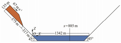
The experiment recorded a series of abundant data, including slide penetration, wave generation, propagation, and run-up, making it a classical illustration to verify the accuracy and performance of numerical simulation methods in assessing LGWs (Quecedo et al., 2004; Biscarini, 2010; Shi et al., 2016; Tan and Chen, 2017). In the present study, the geometry model employed by many scholars (Shi et al., 2016; Tan and Chen, 2017) based on the Lituya LGW experiment by Fritz (2001) was established using an SPH method-based open-source simulator called the DualSPHysics (Crespo et al., 2011; Crespo et al., 2015), which also incorporated the HBP rheological model. The scale of the numerical model is depicted in Fig. 1. Notably, the intersection point of the static water surface and the slope is defined as the coordinate origin. A numerical wave gauge is placed at x = 885 m to monitor the wave fluctuation during the whole process.

The distance between particles is set as 2 m, which eventually creates 15060 nonNewtonian fluid particles for the landslide and 35754 Newtonian fluid particles for the water body. The general SPH configuration parameters for the case are illustrated in Table 1, and details of the parameters for the multiphase flows are presented in Table 2. In Table 2, the initial velocity of 67 m s⁻¹ is applied to the slide body, similar to the experiment configuration, while the density of the slide is set to 2640 kg m⁻³. The rheological parameters of the HBP model, such as yield stress τ_y, viscosity μ, exponent number n, and parameter m, are determined via inverse analysis.

4.1.2 Simulation results

Considering the instance in which the landslide front impacts the water surface, t = 0, we obtain the simulation sequences of the LGW compared with the simplified Lituya LGW experiment by Fritz (2001). As shown in Fig. 2, the whole process of the LGW could be divided into several stages, from landslide-water impact to wave propagation.

ⅰ) Impact stage: The slide rushes quickly along the slope onto the water surface, with the front penetrating into the water, pushing the water rise above the still level into a toe-like shape. Splashes are observed around the boundary of the rising water due to the high-velocity induced impact, and the sharp front of the slide can no longer be maintained as the thickness continues to increase, as shown in Figs. 2(a) – (c).

ⅱ) Cavity creation: The displaced water volume increases as the landslide travels further, and the slide mass tends to become flattened on the bottom. The flow separation on the rock surface due to fast slide penetration creates a large cavity in the interaction zone, as shown in Figs. 2(d) – (h).

ⅲ) Wave generation: As the slide reaches its maximum run-out, the cavity collapses under the gravity effect, generating the leading waves away from the impact zone, as shown in Figs. 2(i) – (l). The visualization of the simulation sequences shows good consistency with the Lituya LGW experiment in terms of the free water surface and landslide dynamics. These findings, therefore, demonstrate the accurate reproduction of deformable LGW by the HBP-based SPH method.

4.1.3 Comparison and validation

In both the experiment and simulation, the results show that the morphological features of the slide have undergone significant changes from its sliding to termination. Specifically, Figs. 2(c) – (e) show that the length of the landslide at the slope foot is shortened for extruding, and its thickness becomes larger. Subsequently, the landslide extends along the channel, becoming longer and thinner until it finally comes to rest, as shown in Figs. 2(f) – (l). Furthermore, as shown in Table 3, the horizontal travel distances between the landslide front and the origin at different instants were compared, and the results revealed great similarities in slide kinematics.

However, the results of the numerical simulation and experiment after 15 s show slight differences. A couple of possible reasons may lead to these differences. First, the fluid in the SPH formalism defined in the current study is treated as weakly compressible, and an equation of state is used to determine the pressure based on particle density. Thus, the pressure has some deviations compared with that observed in the actual case. The deviated pressure term will, in turn, affect the acceleration calculated for the particles, as shown in Eqs. (11) and (9). Second, as the landslide plugs into the water body, the waves become increasingly dispersive, resulting in the uneven distribution of particles in some regions. Given that SPH is a particle-based method, integration error may appear if insufficient neighbor particles meet.

The wave generated by a landslide is formed by the rapid transfer of landslide momentum into the water. The kinetic energy given by the landslide is only partially transformed into the potential energy of uplifting, whereas a considerable part of that is exerted on the water body in the form of a velocity field (Fritz, 2002). The velocity field distribution of the water body pierced through by the landslide is shown in Fig. 2. As shown in the figure, the water velocity field is redistributed with the change of the shape and speed of the slide, indicating that the velocity and deformation of landslide play a critical role in the distribution characteristics of the water velocity field.

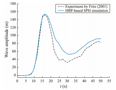
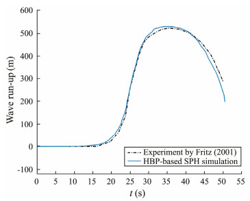
Next, we analyzed the wave amplitude at x = 885 m and wave run-up on the opposite bank to validate the accuracy and applicability of the method in predicting the characteristics of near-field waves caused by deformed landslides. The results are shown in Figs. 3 and 4, respectively. With the wave propagating away from the impact zone to the monitoring position, the first peak of the wave appears at t = 16 s with a maximum amplitude reaching 156 m. This value is considerably close to the maximum amplitude of 152 m obtained in Fritz's experiment. The illustration of the wave run-up on the opposite bank in Fig. 4 also demonstrates great consistency with the data obtained in the experiment, with a maximum run-up of 530 m. The comparison validated that incorporating the HBP rheological model into the SPH method can lead to the accurate representation of the deformable LGWs. Thus, it can be used in practice case analyses.

4.2 Case 2: The Practical Gongjiafang LGW 4.2.1 Overview

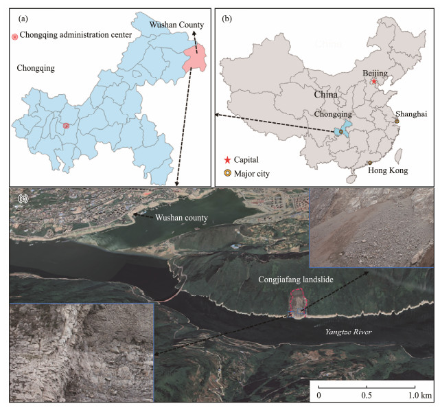
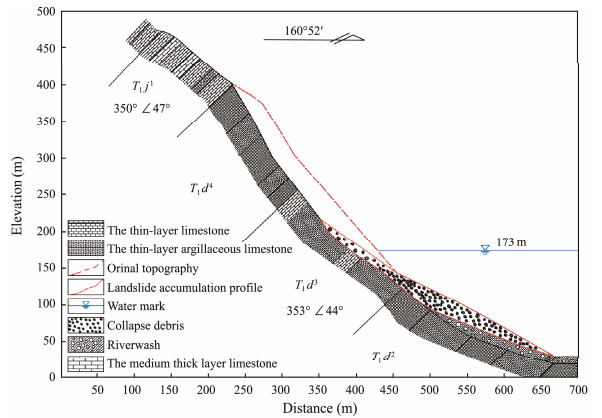
The Gongjiafang landslide is located in Wushan County, Chongqing City, on the north bank of the Yangtze River and within the Wu Gorge of the Three Gorges Reservoir in China (Fig. 5). The study area belongs to the deeply cut river valley landform of middle and low mountains. The slope elevation is about 510 m, with an azimuth of 160˚ and a dip of 50˚ – 70˚. Its bedrock is mainly Lower Triassic horizons primarily composed of the 2nd group (T₁d ²), 3rd group (T₁d ³), and 4th group (T₁d ⁴) of the Daye Formation and the 1st group (T₁ j¹) of the Jialingjiang Formation. The lithology consists of thin-layer argillaceous limestone, limestone, and dolomitic limestone mixed with shale. The orientation of the strata is in the range of 350˚ – 353˚ ∠ 44˚ – 47˚. The rock mass is cut by two groups of main structural planes with orientations of 130˚ – 170˚ ∠ 50˚ – 70˚, and 210˚ – 240˚ ∠ 70˚ – 85˚, which are widely distributed within the rock mass, resulting in the intact rocks breaking into a cataclastic granular structure (Fig. 6).

The landslide occurred on November 23, 2008, when rainfall and rising water levels increased the pore water pressure. The mass released by the collapse with a volume in the order of 38 × 10⁴ m³ entered the river, provoking a maximum wave of 31 m that swept the upstream, down-stream, and other side of the pier. Fortunately, no ships passed by during this period, so no casualties were recorded (Huang et al., 2012). The field investigation found that the failure mass mostly consisted of blocks and debris with an average particle size of 20 cm, as well as many fine particles. In addition, the original reverse slope structure of the interbedded medium-thick limestone and thin argillaceous limestone was completely destroyed (Fig. 5(c)). The above observations indicate that the landslide was seriously disintegrated during the failure process, and its initial structure and morphology were totally violated. Furthermore, many studies revealed that the movement of the landslide along the way showed high mobility with a flow regime (Xiao et al., 2015).

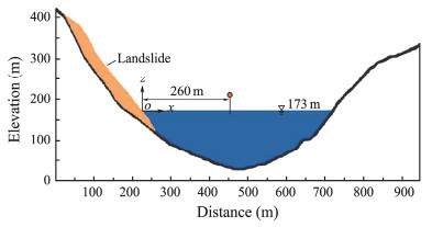
4.2.2 Model configuration

As shown in Fig. 7, a 2D numerical model is established in accordance with the typical geological section. The HBP-based SPH method was applied to analyze the landslide dynamics and near-field LGW features of this event. The particle spacing was fixed at 2 m in the numerical model, resulting in a total number of 17199 particles, including 1325 nonNewtonian particles for the sliding debris, 11670 Newtonian fluid particles for the water body, and 4204 solid boundary particles. As the density of the rock mass of the Gongjiafang slope ranges from 2500 to 2700 kg m⁻³ (Huang and Dai, 2014), the average density was set at 2600 kg m⁻³ in the simulation. The rheological parameters employed for the HBP-based SPH simulation are listed in Table 4.

4.2.3 Results

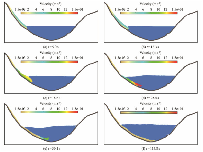
The typical simulation sequences of the Gongjiafang LGW with the color bar indicating the landslide velocity are shown in Fig. 8. As shown in the figure, the shape of the landslide has experienced significant changes from initiation, impact, and up to termination. Furthermore, the landslide front compresses, and the thickness increases from initiation to acceleration, as shown in Figs. 8(a) – (b). Then, as the majority of the slide mass enters the river, the velocity of the landslide gradually decreases due to the combination effect of bottom friction, buoyancy, and drag force of the water. During the process, the shape of the landslide is gradually elongated, wherein the length of the landslide increases to 545 m from 346 m in its initial state, as shown in Figs. 8(c) – (e). Finally, the landslide reaches its termination, and about 80% of the landslide mass is accumulated in the river bottom (Fig. 8(f)).

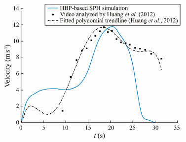
The entire process of the Gongjiafang landslide occurrence was recorded by a local witness whose video clip has been used in previous studies to interpret landslide dynamics and wave amplitude. Huang et al. (2012) extracted the movement of the Gongjiafang landslide by visually analyzing the video. The displacement of the landslide's trailing edge was observed from the video recorded, and its velocity was quantified. The green dots in the figure show that, upon simulation, the average velocity of the landslide at the water inlet varied with time (Fig. 9). The comparison also reveals that the velocity of the landslide has the same variation with time as the maximum velocity (about 11.7 m s⁻¹) during the strong slide-water interaction period (10 s < t < 25 s). However, some differences are observed between the post deceleration stage and the prestage in terms of the landslide dynamics. Before t = 10 s, the simulated landslide velocity is greater than the interpretation by the video. When t > 25 s, the simulation implies that the landslide velocity dramatically drops in a short period, whereas the video interpretation reveals that the landslide gradually decelerates after the peak. This difference can be attributed to the low resolution and absence of scale reference in the video. Furthermore, widespread landslide dust may have led to visual errors in video analysis. Nevertheless, the main kinematic features of the Gongjiafang landslide are well reproduced by the HBP-based SPH simulation, thus proving the effectiveness of the proposed method for practical deformable landslide modeling.

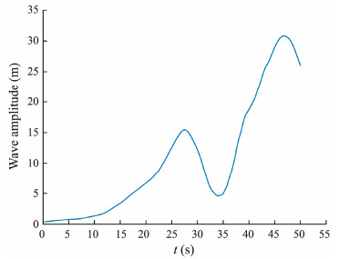
In addition, the characteristics of near-field impulsive waves of this LGW event were considered in this study. To monitor the wave amplitude, a wave gauge was placed at x = 260 m, and the coordinate origin was defined as the intersection of the initial still water and the ground of the landslide (Fig. 7). The numerical result of the wave amplitude time history of this point is presented in Fig. 10. As can be seen, the generated wave appears at an amplitude of 15 m at t = 26 s. It reaches maximum amplitude at approximately 30.7 m above the still water level at t = 47 s, which is very close to the wave amplitude estimated by the video (about 31.8 m) produced by Huang et al. (2012). The above comparison demonstrates that the near-field wave characteristics, especially the maximum wave amplitude, can be captured accurately for practical cases by the proposed method.

5 Discussion 5.1 Effect and Determination of the Rheological Parameters

In general, apart from the geometry settings, the kinematic features of the deformable landslide and the consequent near-field wave characteristics are closely related to the rheological parameters employed when using the HBP model. In the model, there are four crucial parameters that control the dynamic behavior of the nonNewtonian flow (parameter m, exponent number n, consistency index μ_H, and yield stress τ_y). The following section analyzes the effects of the abovementioned parameters on landslide behavior, and the process of determining these parameters is also discussed.

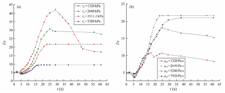
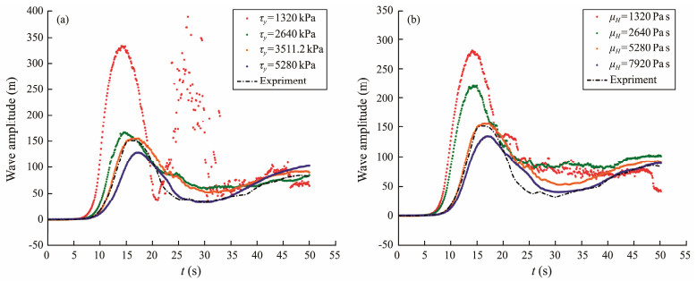
The effects of parameters τ_y and μ_H on the landslide dynamics are shown in Fig. 11, taking the same model as Case 1 for illustration. It can be observed that the deformation degree of the landslide increases with the decrease of yield stress during the interaction process (0 < t < 30 s). In addition, more time is required to reach the termination of the landside with the decrease of yield stress, thereby implying higher velocity. Notably, in the case of τ_y =1320 kPa, the landslide is highly mobilized, inducing mass climbs to the opposite slope and bending up, which is manifested as the decrease in the length-thickness ratio after t = 30 s in Fig. 11(a). As the leading edge of the landslide bends up when it collides with the water body, a larger cavity is produced, resulting in greater wave amplitude (Fig. 12(a)) and a higher run-up (Fig. 13(a)).

Regarding μ_H, it has the same manner as that of τ_y. In the case of a smaller μ_H, the landslide is less viscous and is more likely to be stretched and lengthened, as shown in Fig. 11(b). In the case of a larger μ_H (i.e., μ_H = 7920 Pa s), the tail of the landslide stops at the slope toe, while the leading front is elongated forward, similar to the experimental results. Furthermore, the smaller μ_H induces a stronger pushing effect of the landslide front on the water body, generating higher wave amplitude (Fig. 12(b)) and wave run-up (Fig. 13(b)).

As for practical cases, it is crucial to determine the rheological parameters for the simulation. The most direct and reliable method to do so is to fit the data in accordance with the experimental results, which is a process that requires detailed rheological experimental data and may thus be difficult to implement. Therefore, empirical methods are required to determine the parameters. As an example of a flow-type landslide, several methods for determining rheological parameters for debris flow are summarized through experiments. Here, τ_y and μ_H are considered to be dependent on the mud concentration of a given size (Komatina and Jovanovic, 1997; Von Boetticher et al., 2016). Although the rheological parameters of the HBP model can be obtained using this method, certain conditions, such as the correct particle size or mud concentration, must be met. As for the particle-dominated deformable landslide, the water content is very small, which is different from the debris mixtures.

Nevertheless, studies have suggested referring to some empirical value range or theoretical laws to reverse analysis of relevant parameters by trial-and-error method. In reproducing Fritz's experiment, we obtained m and μ_H by referring to the value of loose sediment in the simulated dam-break test by Fourtakas and Rogers (2016). As for τ_y, this was roughly determined according to the Mohr-Coulomb yield criterion (Dai et al., 2014; Huang and Dai, 2014; Wang et al., 2016a; Han et al., 2022) given by

$ {\tau _y} = c + \sigma \tan \phi, $

(24)

where c is the cohesion, σ is the normal stress that can be assured as the thickness of the initial landslide, and φ is the angle of internal friction. In addition, the exponent number n represents the shearing behavior of the deformable mass. It has been suggested that n = 0.15, −0.9 is suitable for shear-thinning materials, such as the small-size particle-dominated flow mass (i.e., silt, clay), whereas n = 1.0, −3.3 is recommended for granular-dominated shear-thickening mass (Major and Pierson, 1992).

5.2 Merits and Limitations of the HBP Model

As for the HBP model, it is considered a generalized viscoplastic mode for nonNewtonian fluids and is more detailed than the Bingham plastic model. It also eliminates the divergence of the particle system when materials are at the state of having a low shear rate by introducing a continuous function, which is likely to occur when the granular or the slide halts. In addition, the nonlinear behavior of shear stress to shear rate under a high shear strain rate can be accurately described, which means it is more applicable for the modeling of shear-thinning and shear-thickening mixtures than the Bingham and Cross models (Shao and Lo, 2003; Wang et al., 2016a).

However, recent studies have reported that the single phase-based rheological models (i.e., Bingham, HBP, and Cross) are derived from dilute suspensions and rarely consider the volume concentration of solid materials in a mixture. This is a major shortcoming for simulating the granular flow movement, especially if the interstitial fluid pressure dominates the dynamics of the mixture (Si et al., 2018).

Nevertheless, many published studies have adopted the HBP model for modeling the movement of granular materials (Shakibaeinia and Jin, 2011; Fu and Jin, 2015; Fourtakas and Rogers, 2016; Kheirkhahan and Hosseini, 2018; Han et al., 2019, 2020) due to its simplicity and the need to determine fewer rheological parameters. Furthermore, these kinds of single phase-based rheological models are particularly effective and widely adopted for assessing SPH-based particle systems under the Lagrangian framework.

Regarding the LGW problem, the wave characteristics, including the wave amplitude, propagation, and run-up, are key factors to consider. This is because they are closely related to the momentum and energy transfer during the impact stage rather than the interior fluid interacting with the solid fraction of the landslide body during the movement. Nevertheless, the full two-phase models, such as the Eulerian-Eulerian two-phase model based on a collisional-frictional law (Si et al., 2018) and the inertia- and friction-based μ(I) model (Jop et al., 2006; Hosseini et al., 2019), could be applied to simulate impulsive waves triggered by dense granular landslide for comparison study and further improvement in future research.

6 Conclusions

In this study, an HBP-based rheological model that simulates viscous flow is introduced to study the near-field impulsive waves generated by deformable landslides. Under the SPH framework, the impulsive waves generated by deformable landslide is realized by multiphase flow interactions, which is applicable in analyzing the landslide dynamics and predicting near-field impulsive waves.

To verify the accuracy and performance of the proposed model, an experimental case and an engineering case are reproduced and compared with experiment and field observations, respectively. The comparison studies reveal that the simulation results are in good agreement with the case data in terms of landslide dynamics and near-field wave characteristics. Finally, the effects of key parameters in the HBP model on the dynamic behaviors of landslides and the characteristics of near-field waves are also discussed. Tests employing different levels of yield stress and consistency index indicate that the rheological parameters have a significant influence on the landslide dynamics, which, in turn, affect the wave features. Furthermore, the proper determination of the parameters is a challenging but important task. The suggested methods to define the relevant parameters are presented for further practical applications.

Acknowledgements

This study received financial support from the National Natural Sciences Foundation of China (Nos. 42177159, 42077277, 41877253), and the Fundamental Research Funds for the Central Universities, China University of Geosciences (Wuhan) (No. CUG2106304). The support is gratefully acknowledged.