2) School of Atmospheric Sciences, Nanjing University, Nanjing 210023, China
As a part of the cryosphere, sea ice plays an important role in the global climate system (Budyko, 1969). Because of its unique physical and optical characters, sea ice greatly impacts the global climate system through various non-linear dynamic and thermodynamic processes and feedback mechanisms, especially in the following areas: 1) As the interface between the ocean and the atmosphere, sea ice represents an obstacle to air-sea exchanges of heat, momentum, and substances such as CO2 (Rysgaard et al., 2009; Lovely et al., 2015); 2) through the fresh water budget and dense water formation resulting from its melting and freezing, sea ice strongly influences the formation of oceanic deep water, which is one of the driving forces behind the global thermohaline circulation (Levermann et al., 2007; Jahn and Holland, 2013; Ding and Zhang, 2015); and 3) due to its high albedo, sea ice reflects more solar radiation than does sea water and, in turn, reduces the energy absorbed by polar regions (Walsh, 1983; Stephens et al., 2015).
Studies show that, while the balance between the growth and decay of the Arctic sea ice has been broken as a result of extensive melting in recent decades, the ice-albedo feedback mechanism has led to an Arctic amplification of the global warming system and accelerated sea ice reduction (Doscher et al., 2014). In this case, sea ice can impact the atmosphere in nonlinear ways at various scales. For example, a complicated link has been determined between the Arctic sea ice and mid-latitude weather and climate (Budikova, 2009; Cohen et al., 2014; Mori et al., 2014; Walsh, 2014; Vihma, 2014; Gao et al., 2015; Kug et al., 2015; McCusker et al., 2016; Nakamura et al., 2016).
Observations show that the Arctic sea ice has undergone substantial changes within the past few decades (Meier et al., 2014); in fact, current trend has become more negative than ever before (Parkinson and Cavalieri, 2008; Cavalieri and Parkinson, 2012). While global climate models (GCMs) are important tools applied widely to understand the climate and predict climate change, they fail to capture the actual evolution of the Arctic sea ice. Studies from the most recent model simulations of the World Climate Research Programme (WCRP) Coupled Model Intercomparison Project Phase 5 (CMIP5) reveal that nearly all of the trends of the Arctic sea ice extent in September simulated by individual models are lesser than the observed trend (Stroeve et al., 2012). Qiu et al. (2015) evaluated simulations of the Arctic sea ice from the Beijing Climate Center Climate System Model (BCC_CSM) and 14 other CMIP5 models and found that the former simulates too much (little) ice in winter (summer). The sea ice thickness in summer simulated by BCC_CSM is also thinner than that found in actual observations (Tan et al., 2015). These shortcomings are mainly related to two aspects: the imperfections of the related sea ice model and the inaccuracy of the external forcing from atmosphere and ocean components of BCC_CSM. To address these issues and improve the performance of BCC_CSM in polar regions, the Los Alamos sea ice model (CICE) developed by the Los Alamos National Laboratory was introduced to BCC_CSM as an alternative to the Sea Ice Simulator (SIS) (Fang et al., 2017). Compared with the original version of this model, several important parameters were adjusted and verified (Chu et al., 2018). CICE is more complex than the original sea ice component in BCC_CSM because it features up-to-date physical processes, which will be introduced later. After coupling work, assessment of the basic performance of the model in Arctic climate simulations is necessary and indispensable. In general, the proper approach to this target is to run BCC_CSM with the two sea ice components separately while keeping all other settings identical; this approach reduces the influence of other factors and focuses on the impacts of the sea ice process on the climate system.
In this paper, the performance of BCC_CSM with SIS and CICE in Arctic sea ice simulations and the impacts of these components on polar climate are evaluated. The remainder of this paper is organized as follows. The BCC_CSM and its sea ice components are introduced, and descriptions of the settings for experiments and observations used for model evaluation are provided in Section 2. Then, evaluation and comparison of the simulation results obtained from the two sea ice component models are conducted in Section 3. Section 4 completes the main text with a discussion and conclusions.
2 Model and Experiments 2.1 Model DescriptionThe BCC_CSM (Wu et al., 2014) is a fully coupled climate system model developed by the Beijing Climate Center and consists of four components: the atmospheric circulation model BCC_AGCM2.0 (Wu et al., 2010), the ocean circulation model MOM4 (Griffies et al., 2005), the land surface process model BCC_AVIM2.0 (Wu et al., 2014), and the sea ice model. These component models are coupled together through the National Center for Atmospheric Research (NCAR) coupler version 5 (Kiehl and Gent, 2004). A thorough introduction of these components, including their physical settings and performance, is provided in the above references.
The original sea ice component model of BCC_CSM is SIS (Winton, 2000), which was developed by the Geophysical Fluid Dynamics Laboratory. SIS is a global dynamical-thermodynamical sea ice model in which the elastic-viscous-plastic (EVP) technique (Hunke and Dukowicz, 1997) is used to calculate ice internal stresses, and the thermodynamic component employs a scheme by Winton (2000) modified from Semtner's three-layer frame- work (Semtner, 1976). SIS features three vertical layers, including one layer of snow cover and two layers of equally sized sea ice. In each model grid, five categories of sea ice are considered according to the sea ice thickness.
CICE is another sea ice component model that has been coupled to BCC_CSM. CICE considers more complex physical processes than SIS. It includes a subgrid-scale ice thickness distribution (Lipscomb, 2001), energy-conserving thermodynamics (Bitz and Lipscomb, 1999), which features multiple vertical layers and accounts for the thermodynamic influences of brine pockets within the ice cover, EVP dynamics (Hunke and Dukowicz, 1997), and an improved ridging scheme (Lipscomb et al., 2007). CICE adopts the Delta-Eddington radiative scheme (Briegleb and Light, 2007) and level-ice melt pond scheme (Hunke et al., 2013) which enable it to treat surface albedos with great sophistication and internal consistency. Compared with SIS, CICE features more and tunable vertical layers for snow and sea ice. A detailed comparison of the CICE and SIS models is provided in Table 1.
|
|
Table 1 Comparison of the sea ice models SIS and CICE |
The basic model configuration adopted in this paper is described in this section. BCC_AGCM2.0 and BCC_AVIM2.0 have identical horizontal resolutions of approximately 2.8° (T42, 128 × 64 grids globally). BCC_AGCM 2.0 has 26 vertical levels. The ocean model MOM4 has a horizontal resolution of about 1° longitude by 1/3° latitude (between 10°S and 10°N) ranged to 1° latitude (at 30°N and 30°S) and nominally 1° polarward with tri-polar coordinates. MOM4 has 40 levels in the vertical direction. The horizontal resolution of the sea ice model is identical to that of MOM4.
Two simulation experiments are designed under the framework of BCC_CSM; in these experiments, the same configurations are employed but the sea ice component differs: one case uses SIS and the other uses CICE. Since the ocean and sea ice component models require some time to reach equilibrium, we apply two phases to run the models. In the first step, we run the circulation model by integrating BCC_CSM for 50 model years with external forcing in the year 1950, including greenhouse gases, ozone, aerosols, volcanoes and solar variability. As the model approaches its quasi-equilibrium state, we continue to run the model from 1950 to 2012 with temporally evolving forcing. In this paper, we mainly compare the CICE and SIS experiments against observations of the climate mean from 1981 to 2005, which are taken as a representative of the present-day climate.
2.3 Observation DatasetsDue to the lack of available observations on the polar region, datasets from satellite remote-sensing and reanalysis data from model simulations and assimilation systems are used for model evaluation in this paper.
The Met Office Hadley Centre Sea Ice and Sea Surface Temperature (HadISST; Rayner et al., 2003) datasets are used to describe sea ice concentrations and sea surface temperatures (SST). Sea ice extent (SIE) data are obtained from the National Snow and Ice Data Center (NSIDC) climatology dataset for the period 1981–2005 (https://svn-ccsm-moels.cgd.ucar.edu/tools/proc_ice/trunk/ice_diag/ice_diag_trunk/data/SSMI.ice_extent.1981-2005.monthly.regional.txt). Sea ice thickness data are obtained from the ORAP5 (Ocean ReAnalysis Pilot 5) reanalysis from the European Center for Medium-Range Weather Forecasts (ECMWF; Tietsche et al., 2014). Datasets from the National Centers for Environmental Prediction Reanalysis 2 (NCEP2; Kanamitsu et al., 2002) and the Japanese 55-year Reanalysis (JRA55, Kobayashi et al., 2015) are also used to analyze the polar atmosphere, including surface air temperature, sea level pressure (SLP), and other surface parameters.
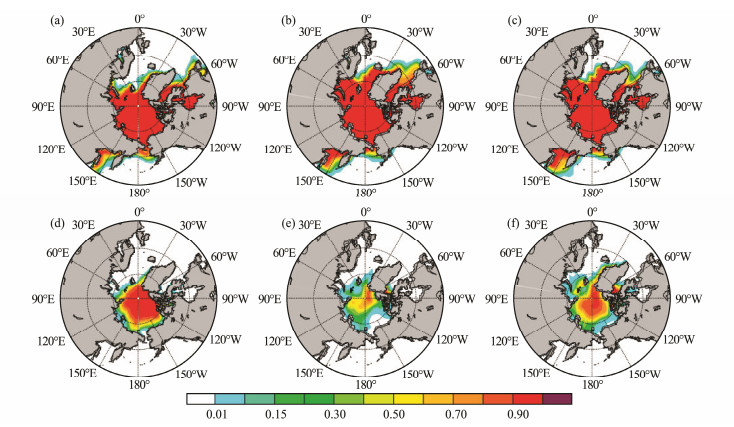
3 Simulation Results Analysis 3.1 Arctic Sea IceThe most important and primary parameters of sea ice are its concentration and thickness. Here, we first evaluate the spatial distributions of sea ice in representative months of winter and summer. The peak Arctic SIE occurs in March. As shown in Fig. 1, the Arctic Ocean, the Okhotsk Sea, the Barents Sea, and the Kara Sea are all covered by sea ice with concentration levels above 90% (Fig. 1a). Simulations with the SIS and CICE component models reproduce reasonable ice concentration distributions in the Arctic region, and differences between the two experiments are generally small, expect in the Labrador Sea (Figs. 1b and 1c). Compared with the Hadley observation data, the main discrepancies of BCC_CSM include overestimation of the ice simulated in the regions of the Okhotsk Sea and Greenland/Iceland/Norwegian (GIN) Sea, which is likely due to biases from the modeled ocean surface conditions (Tan et al., 2015). The minimum Arctic SIE is observed in September, during which the sea ice retreats to the Arctic Ocean basin (Fig. 1d). The sea ice distributions simulated by CICE are clearly much closer to actual observations than those simulated by SIS (Figs. 1e and 1f). SIS generally underestimates the summer sea ice distribution, especially in the Barents Sea, the Beaufort Sea, and even the central Arctic Ocean, where small amounts of ice and a low ice concentration are present.
|
Fig. 1 Observed and simulated mean Arctic sea ice concentrations for the period 1981–2005 in March (a, b, c) and September (d, e, f). (a, d), Hadley's observations; (b, e), SIS simulations; and (c, f), CICE simulations. |
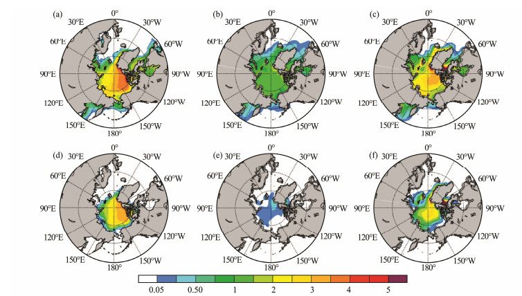
The simulated sea ice thickness and corresponding observations are shown in Fig. 2. Observations in March and September reveal that the thickest sea ice is located in the northern coast of Greenland and the Canadian Archipelago and there is a negative gradient to thinner ice at the Siberian coast. In March, the thickest ice observed is about 4–5 m-thick, and the thickness of sea ice in the Arctic Basin varies from 2 m to 4 m (Fig. 2a). The thickness simulated by the SIS model shows a relatively flat distribution pattern with thicknesses ranging from 1 m to 2 m (Fig. 2b). Comparatively, the sea ice thickness simulated by CICE is generally larger than that determined by SIS and ranges from 2 m to 4 m (Fig. 2c). Therefore, the sea ice simulated by the SIS model is thinner by as much as 2 m compared with actual observations and the results of the CICE experiment. This situation gets worse in summer as thin ice is easier to melt than thick ice. As a result, the ice thickness simulated by the SIS experiment in September is thinner than 20 cm (Fig. 2e) while the observation shows a 2–3 m thickness distribution (Fig. 2d). The CICE simulation results (Fig. 2f) are much closer to actual observations than the SIS results, although some biases are detected in the Davis Strait, where the sea ice thickness is overestimated by more than 5 m. This issue is most probably related to insufficient advection toward lower latitudes due to the model geography. Therefore, the sea ice thickness is better reproduced in BCC_CSM simulations with the CICE model than in those with the SIS model.
|
Fig. 2 Observed and simulated mean Arctic sea ice thickness for the period 1981–2005 in March (a, b, c) and September (d, e, f; Unit: m). (a, d), ORAP5 observations; (b, e), SIS simulations; and (c, f), CICE simulations. |
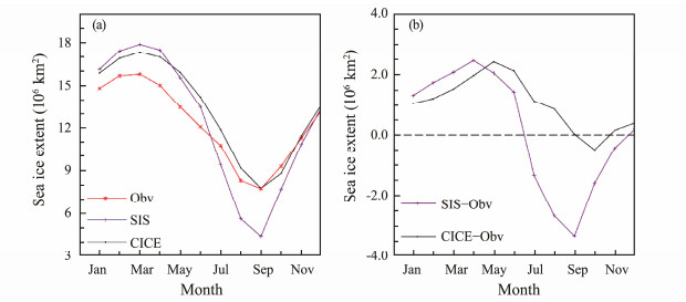
To evaluate the simulated temporal evolution of sea ice cover, we calculated the Northern Hemisphere SIE, which is defined as the total area of ice model grids with a sea ice concentration above 15%. Observations from NSIDC show that the Arctic sea ice cover has a minimum extent of 7.74×10⁶ km2 in September and a maximum extent of 15.79×10⁶ km2 in March (red line in Fig. 3a). Simulations with the SIS and CICE models capture the seasonal variation and pattern very well, but remarkable differences exist in the magnitude. The simulated SIEs obtained from the SIS model are greater than actual observations from January to June and smaller from July to December, reaching 17.87×10⁶ and 4.41×10⁶ km2 in March and September, respectively (purple line in Fig. 3a). By comparison, experiments with CICE reveal a maximum ice extent of 17.32× 10⁶ km2 in March and a minimum extent of 7.77×10⁶ km2 in September (black line in Fig. 3a), which is closer to actual observations than those produced by SIS. Differences in SIEs between the two simulations and NSIDC observations illustrated in Fig. 3b clearly indicate that experiments with CICE return smaller deviations than those with the SIS model in most of the months. The most remarkable improvements of CICE compared with SIS appear in warmer seasons, especially in September, with the deviation in SIE decreasing from 3.33×10⁶ to 0.03×10⁶ km2. However, SIS and CICE share some common weaknesses, such as overestimation of sea ice in winter. This may be a result of exterior forcing or interior physical processes in the sea ice models. More studies should be carried out to determine what is causing this discrepancy and how to improve on it. From the above analysis, the CICE in BCC_CSM clearly shows better performance than SIS in Arctic sea ice simulations, which is consistent with previous studies (e.g., Behrens et al., 2012; Stroeve et al., 2012).
|
Fig. 3 (a) Observed and simulated mean seasonal cycles of the Arctic SIE and (b) biases between the simulations and actual observations. (a), the red line denotes NSIDC observations; the purple line denotes SIS simulation; and the black line denotes CICE simulation. (b), the purple line denotes biases between the SIS simulation and observations, while the black line denotes biases between the CICE simulation and observations. |
The simulations with the CICE component in BCC_CSM show greatly improved model performance in terms of sea ice concentration, thickness, and seasonal cycle of the Arctic SIE. These improvements will, in turn, affect the energy transformation between the climate system components of the atmosphere, ice, and ocean. Changes are anticipated to appear in the simulated atmosphere and ocean climate. Therefore, in this section, the influences of the two sea ice models on the Arctic climate are analyzed.
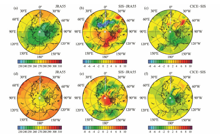
The spatial distribution of surface air temperatures is first evaluated. In March, the observed temperatures on ocean are higher than those on land at the same latitude and decrease rapidly from low-latitude areas to the Arctic Ocean; the coldest region appears in Greenland (Fig. 4a). Differences between JRA55 data and the SIS simulation results reveal significant deviations in some regions. Negative (cold) biases appear in the Okhotsk Sea, as well as the Greenland Sea, Barents Sea and Labrador Sea, while positive (warm) biases appear in the Beaufort Sea, Central Arctic, and Baffin Bay (Fig. 4b). The negative bias is mainly due to the positive bias afforded by the sea ice cover shown in Fig. 1. Since the Barents Sea and Northwest Pacific are key regions in which intensive loss of heat from the ocean occurs, the presence of sea ice blocks heat release from the ocean to the atmosphere and results in cooling of these regions. Additionally, weak North Atlantic current contributes to cold biases in the Greenland Sea and Barents Sea (figures not shown). Simulations with CICE yield generally reduced deviations compared with those of SIS, as shown in Fig. 4c. Thus, warm biases in the Arctic Ocean and cold biases in the Barents Sea and the Greenland Sea are effectively diminished.
|
Fig. 4 Mean surface air temperatures in March (a, b, c) and September (d, e, f) for the period 1981–2005 (Unit: K). (a, d), observational estimates from JRA55; (b, e), differences between the SIS experiment and actual observations; and (c, f), differences between the CICE and SIS experiments. |
In September, the most notable features of surface temperature determined through BCC_CSM simulations with SIS are a large warm bias of up to 8℃ over the whole Arctic Ocean and Greenland and a cold bias of up to 5℃ in the North Atlantic and Pacific Oceans (Fig. 4e). By contrast, experiments with CICE show better performance, with lower temperatures in most parts of the Arctic Ocean and higher temperatures in those negative regions determined from the SIS experiment, except in the Okhotsk Sea (Fig. 4f). These improvements can be mainly attributed to the accurate reproductions of sea ice concentration and thickness provided by the CICE model. However, simulations with CICE reveal colder biases in the Okhotsk Sea compared with those obtained from SIS.
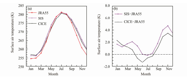
The temporal evolution of regional mean surface temperatures is further analyzed. As presented in Fig. 5, the seasonal cycle of surface air temperatures (from 45° to 90°N) are well captured by BCC_CSM simulations with the two sea ice models, although magnitude differences are observed. The two experiments show larger (smaller) biases in cold (warm) seasons compared with actual observations, but the CICE experiment matches the JRA55 observations better than does the SIS experiment in most months, except in January and February.
|
Fig. 5 (a) Observed and simulated mean surface air temperature in regions 45°N–90°N for the period 1981–2005 (Unit: K) and (b) biases between the simulations and actual observations. (a), the red line denotes JRA55 observations; the purple line denotes SIS simulation; and the black line denotes CICE simulation. (b), the purple line denotes biases between the SIS simulation and observations, while the black line denotes biases between the CICE simulation and observations. |
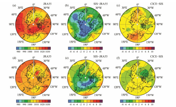
Sea level pressure (SLP) is also an important and basic climatic variable for evaluating atmospheric circulation. Fig. 6 illustrates the SLP spatial distributions from JRA55 and BCC_CSM simulated results. In March, observations indicate major winter atmospheric activity centers in Arctic areas, including the Icelandic Low, Aleutian Low, Siberian High, and Beaufort High (Fig. 6a). Compared with observations, the Siberian High and Beaufort High simulated by SIS are weaker, whereas the Aleutian Low and Icelandic Low are significantly stronger (Fig. 6b); these results are somewhat consistent with the bias pattern of surface temperature (Fig. 4b). In addition, the simulated Aleutian Low shifts slightly to the east from its original position, resulting in a lower SST and over-extended sea ice cover in the Okhotsk Sea. Differences among CICE and SIS results in Fig. 6c generally contrast the patterns found in Fig. 6b, which indicates improvements in model performance through incorporation of the CICE component, especially in regions around the Arctic Basin and North Atlantic. These improvements could be mainly attributed to improved spatial distributions of sea ice thickness in CICE (c.f. Fig. 2c) which leads to increased ice albedos and, in turn, decreased net shortwave radiation (figures not shown) and result in lower surface temperatures and higher SLPs in the Arctic; in fact, the Siberian High and the Beaufort High are particularly significantly strengthened. However, it is also notable that the Aleutian Low determined in the CICE experiment is stronger than that in the SIS experiment.
|
Fig. 6 Mean sea level pressure in March (a, b, c) and September (d, e, f) for the period 1981–2005 (Unit: hPa). (a, d), observational estimates from JRA55; (b, e) differences between the SIS experiment and actual observations; and (c, f) differences between the CICE and SIS experiments. |
The main atmospheric activity centers in the Arctic in September are similar to but weaker than those in March (Fig. 6d). The SLP simulated by SIS is significantly lower than that observed in Arctic regions, especially in the East Siberian and Beaufort Seas (Fig. 6e). These biases are largely improved in the CICE experiment (Fig. 6f) along with improvements in sea ice simulations.
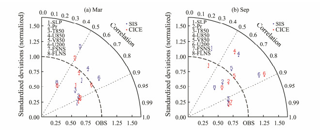
Taylor diagrams provide an efficient and comprehensive visual framework for comparing a suite of variables from model simulations to observational datasets. Here, two Taylor diagrams are shown in Fig. 7 for March and September. Eight variables, including SLP, Pr (precipitation rate), T850 (850 mb temperature), U850 (850 mb zonal wind), V850 (850 mb meridional wind), U200 (200 mb zonal wind), FSNS (surface net SW flux), and FLNS (surface net LW flux), are analyzed; here, the observational data are from the NCEP reanalysis. As each field is normalized by the corresponding standard deviation of the reference observational data, the ratio of the normalized variances indicates the relative amplitude of the model and observed variations.
|
Fig. 7 Taylor diagrams of the geographical distributions of mean atmospheric fields in March (a) and September (b). Blue dots denote SIS experiments, while red dots denote CICE experiments. The numbers present the different atmospheric variables. |
Results show that, for most variables, correlations between model simulations and the corresponding observations range from 0.5 to 0.9. However, the accuracy of the simulations depends on the fields and differs between the two experiments. In March, V850 (number 5 in Fig. 7a) and FLNS (number 8) show the lowest correlations, whereas Pr (number 2) and FSNS (number 7) show the highest ones. In September, SLP (number 1 in Fig. 7b) shows the poorest correlation, whereas T850 (number 3) and FSNS (number 7) show the highest ones. For most fields considered here, the amplitude of spatial variability simulated by the CICE experiment is reasonably closer to observations than that simulated by SIS, except for FLNS (number 8 in Fig. 7a) and SLP (number 1 in Fig. 7a) in March and U200 (number 6 in Fig. 7b) in September.
Changes in sea ice also impact ocean properties. Here, we discuss the sea surface temperature (SST) and Atlantic meridional overturning circulation (AMOC).
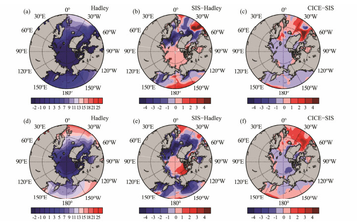
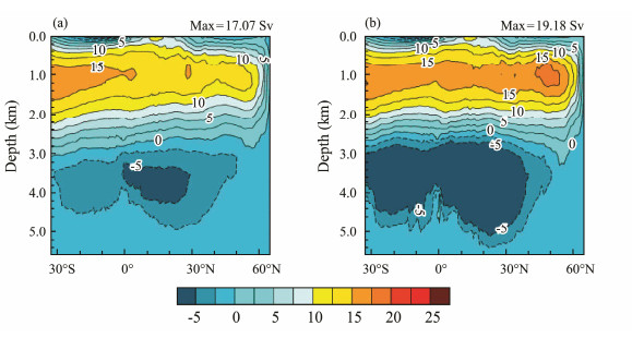
As sea ice is mainly formed from the freezing of surface water, SST is very important for sea ice formation and melting and also affected by sea ice. The spatial distributions of SST are shown in Fig. 8. Compared with Hadley's observations, the SIS experiment in March shows positive biases over the whole Arctic Basin and most of the North Pacific and North Atlantic and distinct negative biases in the Okhotsk, Gulf of Alaska, Barents Sea, and Nordic Seas (Fig. 8b). The CICE experiment shows remarkable differences compared with SIS, especially a colder SST in the Arctic Basin and warmer SST in the North Atlantic, which decreases model errors (Fig. 8c). Differences between the SIS experiment and actual observations in September (Fig. 8e) show similar patterns as in March, i.e., positive in the Arctic Ocean and especially negative at the North Pacific and Atlantic, which are also greatly improved in CICE experiment (Fig. 8f). Improvements in the Arctic Ocean both in March and September benefit from a thicker ice distribution, which, in turn, decreases incident shortwave radiation through the ice to the ocean surface. More importantly, regions with extensive cold anomalies in the North Atlantic are greatly improved. On the one hand, it is a result from improvements in the simulation of sea ice distributions, i.e., smaller SIEs in the regions of interest (c.f. Fig. 1), and on the other hand, it is also related to the stronger AMOC derived from CICE, as presented in Fig. 9.
|
Fig. 8 Mean sea surface temperatures (Unit: ℃) in March (a, b, c) and September (d, e, f) for the period 1981–2005. (a, d), observational estimates from Hadley; (b, e), differences between the SIS experiment and actual observations; and (c, f) differences between the CICE and SIS experiments. |
|
Fig. 9 Annual mean Atlantic meridional overturning stream function (AMOC) from BCC_CSM simulations with SIS (a) and CICE (b). |
AMOC is an important indicator of climate through its heat and freshwater transports. According to observation-based estimates, the average strength of AMOC is about 16.5 Sv at 48°N (Ganachaud, 2003). The annual mean AMOC transport patterns in depth-latitude are shown in Fig. 9. Simulations with SIS and CICE reveal similar and reasonable patterns with high northward transport regions at 1000 m, a surface maximum at 10°–20°N, and a rather strong southward transport at approximately 4000 m. However, the AMOC strength and extent between the two simulations apparently differ. The annual maximum AMOC simulated by CICE within 50°–53°N is up to 17.5 Sv, which is about 5 Sv stronger than that determined from SIS and much closer to observational estimates.
As ice formation and the resulting brine rejection increase salinity, CICE features greater and thicker ice distributions and, as a result, modulates the high-latitude convective and mixing processes involved in the sinking branch of the AMOC. Therefore, the stronger AMOC determined by CICE is likely driven by stronger deep convection across the Nordic seas due to deviations in sea ice characteristics between the two simulations.
4 Discussions and ConclusionsThe sea ice model CICE was introduced to BCC_CSM, and two coupling experiments using SIS and CICE as sea ice component models were conducted with all other settings held same. The impacts of different sea ice component models on the model performance of Arctic sea ice and climate were evaluated. The major conclusions are:
1) In terms of Arctic sea ice, simulations with CICE show better performance than do simulations with SIS on reproducing the spatial distribution and annual cycle of the Arctic SIE. The most encouraging improvements are SIE in September and the sea ice thickness in nearly all seasons. SIS simulations underestimated the sea ice thickness in both winter and summer. For example, the ice thickness determined from SIS simulations in September is thinner than 20 cm; by contrast, CICE presents a 2–3 m thickness distribution, which is closer to observations.
2) Due to the improved performance of simulations of sea ice distribution by CICE, significant improvements in the simulation of the Arctic climate were generally obtained. The warm biases of surface air temperature and SST and lower SLP biases in the SIS experiments are reduced in the CICE simulations. Taylor diagrams for eight atmospheric variables show that CICE yields results that are more reasonable and closer to observations than those produced by SIS in both March and September.
3) Simulations with the CICE model generate stronger AMOC than those with SIS, which indicates better descriptions of the interaction between sea ice and ocean.
Improvements in the model performance on Arctic sea ice and climate with CICE model in BCC_CSM likely benefit from complex physical processes and finer vertical resolutions (Fang et al., 2017). However, we also noted a number of common weaknesses in the SIS and CICE experiments. For example, both components feature a distinct cold bias for surface air temperature and SST and positive bias for sea ice concentration in the Okhotsk Sea in winter. Hence, the seasonal cycle of SIE and temperature should be investigated further. Because of the interactions between sea ice, atmosphere, and ocean, improving sea ice simulations requires improvements in both the atmosphere and ocean components, in addition to upgrades to the sea ice component itself. Therefore, understanding the mechanisms governing sea ice formation and melting in this region is of crucial importance. More experiments and further analysis should be carried out on this topic. In addition, in this paper, we focused on the mean climate state and seasonal cycle and not the interannual variability of the Arctic sea ice, which is also an important but challenging research field that requires further investigation.
AcknowledgementsThis work was jointly supported by the National Basic Research Program of China (No. 2015CB953904), the Welfare Program of Meteorology (No. GYHY201506011), and the National Key R & D Program (Nos. 2016YFA060 2602, 2018YFC1407104).
Behrens, L. K., Martin, T., Semenov, V. A. and Latif, M., 2012. The Arctic sea ice in the CMIP3 climate model ensemble-variability and anthropogenic change. The Cryosphere Discussions, 6: 5317-5344. DOI:10.5194/tcd-6-5317-2012 (  0) 0) |
Bitz, C. M. and Lipscomb, W. H., 1999. An energy-conserving thermodynamic model of sea ice. Journal of Geophysical Research, 104: 15669-15677. DOI:10.1029/1999JC900100 (  0) 0) |
Briegleb, B. P., and Light, B., 2007. A Delta-Eddington multiple scattering parameterization for solar radiation in the sea ice component of the Community Climate System Model. National Center for Atmospheric Research Technical Note NCAR/TN-472+STR. Boulder, Colorado, 1-100.
(  0) 0) |
Budikova, D., 2009. Role of Arctic sea ice in global atmospheric circulation: A review. Global and Planetary Change, 68: 149-163. DOI:10.1016/j.gloplacha.2009.04.001 (  0) 0) |
Budyko, M., 1969. The effect of solar radiation variations on the climate of the earth. Tellus, 21: 611-619. (  0) 0) |
Cavalieri, D. J. and Parkinson, C. L., 2012. Arctic sea ice variability and trends, 1979-2010. The Cryosphere, 6: 881-889. DOI:10.5194/tc-6-881-2012 (  0) 0) |
Chu, M., Fang, Y. J., Zhang, L. J. and Wu, T. W., 2018. Influence of albedo related parameters on the simulation of Arctic sea ice by CICE. Acta Meteorologica Sinica, 76(3): 461-472 (in Chinese with English abstract). (  0) 0) |
Cohen, J., Screen, J. A., Furtado, J. C., Barlow, M., Whittleston, D., Coumou, D., Francis, J., Dethloff, K., Entekhabi, D., Overland, J. and Jones, J., 2014. Recent Arctic amplification and extreme mid-latitude weather. Nature Geoscience, 7: 627-637. DOI:10.1038/ngeo2234 (  0) 0) |
Ding, Y. J. and Zhang, S. Q., 2015. The hydrological impact of cryosphere water cycle on global-scale water cycle. Chinese Science Bulletin, 60(7): 593-602 (in Chinese with English abstract). DOI:10.1360/N972014-00899 (  0) 0) |
Doscher, R., Vihma, T. and Maksimovich, E., 2014. Recent advances in understanding the Arctic climate system state and change from a sea ice perspective: A review. Atmospheric Chemistry and Physics, 14: 13571-13600. DOI:10.5194/acp-14-13571-2014 (  0) 0) |
Fang, Y. J., Chu, M., Wu, T. W., Zhang, L. J. and Nie, S. C., 2017. Coupling of CICE5.0 with BCC_CSM2.0 model and its performance evaluation on Arctic sea ice simulation. Haiyang Xuebao, 39(5): 33-43 (in Chinese with English abstract). (  0) 0) |
Ganachaud, A., 2003. Large-scale mass transports, water mass formation, and diffusivities estimated from World Ocean Circulation Experiment (WOCE) hydrographic data. Journal of Geophysical Research, 108: 3213. DOI:10.1029/2002JC001565 (  0) 0) |
Gao, Y. Q., Sun, J. Q., Li, F., He, S. P., Sandven, S., Yan, Q., Zhang, Z. S., Lohmann, K., Keenlyside, N., Furevik, T. and Suo, L. L., 2015. Arctic sea ice and Eurasian climate: A review. Advances in Atmospheric Sciences, 32(1): 92-114. DOI:10.1007/s00376-014-0009-6 (  0) 0) |
Griffies, S. M., Gnanadesikan, A., Dixon, K. W., Dunne, J. P., Gerdes, R., Harrison, M. J., Rosati, A., Russell, J. L., Samuels, B. L., Spelman, M. J., Winton, M. and Zhang, R., 2005. Formulation of an ocean model for global climate simulations. Ocean Science, 1: 45-79. DOI:10.5194/os-1-45-2005 (  0) 0) |
Hunke, E. C. and Dukowicz, J. K., 1997. An elastic-viscous-plastic model for sea ice dynamics. Journal of Physical Oceanography, 27: 1849-1867. DOI:10.1175/1520-0485(1997)027<1849:AEVPMF>2.0.CO;2 (  0) 0) |
Hunke, E. C., Hebert, D. A. and Lecomte, O., 2013. Level-ice melt ponds in the Los Alamos sea ice model, CICE. Ocean Modelling, 71: 26-42. DOI:10.1016/j.ocemod.2012.11.008 (  0) 0) |
Jahn, A. and Holland, M. M., 2013. Implications of Arctic sea ice changes for North Atlantic deep convection and the meridional overturning circulation in CCSM4-CMIP5 simulations. Geophysical Research Letters, 40: 1206-1211. DOI:10.1002/grl.50183 (  0) 0) |
Kanamitsu, M., Ebisuzaki, W., Woollen, J., Yang, S. K., Hnilo, J. J., Fiorino, M. and Potter, G. L., 2002. NCEP-DOE AMIP-Ⅱ reanalysis (R-2). Bulletin of American Meteorological Society, 83: 1631-1643. DOI:10.1175/BAMS-83-11-1631 (  0) 0) |
Kiehl, J. T. and Gent, P. R., 2004. The community climate system model, version 2. Journal of Climate, 17: 3666-3682. DOI:10.1175/1520-0442(2004)017<3666:TCCSMV>2.0.CO;2 (  0) 0) |
Kobayashi, S., Ota, Y., Harada, Y., Ebita, A., Moriya, M., Onoda, H., Onogi, K., Kamahori, H., Kobayashi, C., Endo, H., Miyaoka, K. and Takahashi, K., 2015. The JRA-55 reanalysis: General specifications and basic characteristics. Journal of the Meteorological Society of Japan, 93(1): 5-48. DOI:10.2151/jmsj.2015-001 (  0) 0) |
Kug, J. S., Jeong, J. H., Jang, Y. S., Kim, B. M., Folland, C. K., Min, S. K. and Son, S. W., 2015. Two distinct influences of Arctic warming on cold winters over North America and East Asia. Nature Geoscience, 8: 759-763. DOI:10.1038/ngeo2517 (  0) 0) |
Levermann, A., Mignot, J., Nawrath, S. and Rahmstorf, S., 2007. The role of northern sea ice cover for the weakening of the thermohaline circulation under global warming. Journal of Cli- mate, 20: 4160-4171. (  0) 0) |
Lipscomb, W. H., 2001. Remapping the thickness distribution in sea ice models. Journal of Geophysical Research Oceans, 106: 13989-14000. DOI:10.1029/2000JC000518 (  0) 0) |
Lipscomb, W. H., Hunke, E. C., Maslowski, W. and Jakacki, J., 2007. Ridging, strength, and stability in high-resolution sea ice models. Journal of Geophysical Research, 112: C03S91. (  0) 0) |
Lovely, A., Loose, B., Schlosser, P., McGillis, W., Zappa, C., Perovich, D., Brown, S., Morell, T., Hsueh, D. and Friedrich, R., 2015. The gas transfer through polar sea ice experiment: Insights into the rates and pathways that determine geochemical fluxes. Journal of Geophysical Research Oceans, 120: 8177-8194. DOI:10.1002/2014JC010607 (  0) 0) |
McCusker, K. E., Fyfe, J. C. and Sigmond, M., 2016. Twenty-five winters of unexpected Eurasian cooling unlikely due to Arctic sea-ice loss. Nature Geoscience, 9: 838-843. DOI:10.1038/ngeo2820 (  0) 0) |
Meier, W. N., Hovelsrud, G. K., Oort, B. E., Key, J. R., Kovacs, K. M., Michel, C., Haas, C., Granskog, M. A., Gerland, S., Perovich, D. K., Makshtas, A. and Reist, J. D., 2014. Arctic sea ice in transformation: A review of recent observed changes and impacts on biology and human activity. Review of Geophysics, 51: 185-217. (  0) 0) |
Mori, M., Watanabe, M., Shiogama, H., Inoue, J. and Kimoto, M., 2014. Robust Arctic sea-ice influence on the frequent Eurasian cold winters in past decades. Nature Geoscience, 7: 1-5. (  0) 0) |
Nakamura, T., Yamazaki, K., Iwamoto, K., Honda, M., Miyoshi, Y., Ogawa, Y., Tomikawa, Y. and Ukita, J., 2016. The stratospheric pathway for Arctic impacts on midlatitude climate. Geophysical Research Letters, 43: 3494-3501. DOI:10.1002/2016GL068330 (  0) 0) |
Parkinson, C. L. and Cavalieri, D. J., 2008. Arctic sea ice variability and trends, 1979-2006. Journal of Geophysical Research, 113: C07003. (  0) 0) |
Qiu, B., Zhang, L. J., Chu, M., Wu, T. W. and Tan, H. H., 2015. Performance analysis of Arctic sea ice simulation in climate system models. Chinese Journal of Polar Research, 27(1): 47-55 (in Chinese with English abstract). (  0) 0) |
Rayner, N. A., Parker, D. E., Horton, E. B., Folland, C. K., Alexander, L. V., Rowell, D. P., Kent, E. C. and Kaplan, A., 2003. Global analyses of sea surface temperature, sea ice, and night marine air temperature since the late nineteenth century. Journal of Geophysical Research, 108(D14): 4407. DOI:10.1029/2002JD002670 (  0) 0) |
Rysgaard, S., Bendtsen, J., Pedersen, L. T., Ramlov, H. and Glud, R. N., 2009. Increased CO2 uptake due to sea ice growth and decay in the Nordic Seas. Journal of Geophysical Research, 114: C09011. (  0) 0) |
Semtner, A. J., 1976. A model for the thermodynamics growth of sea ice in numerical investigations of climate. Journal of Physical Oceanography, 6: 27-37. (  0) 0) |
Stephens, G. L., O'Brien, D., Webster, P. J., Pilewski, P., Kato, S. and Li, J. L., 2015. The albedo of earth. Reviews of Geophysics, 53(1): 141-163. (  0) 0) |
Stroeve, J. C., Kattsov, V., Barrett, A., Serreze, M., Pavlova, T., Holland, M. and Meier, W. N., 2012. Trends in Arctic sea ice extent from CMIP5, CMIP3 and observations. Geophysical Research Letters, 39: L16502. (  0) 0) |
Tan, H. H., Zhang, L. J., Chu, M., Wu, T. W., Qiu, B. and Li, J. L., 2015. An analysis of simulated global sea ice extent, thickness and causes of error with the BCC_CSM model. Chinese Journal of Atmospheric Sciences, 39: 1-13 (in Chinese with English abstract). (  0) 0) |
Tietsche, S., Balmaseda, M. A., Zuo, H., and Mogensen, K., 2014. Arctic sea ice in the ECMWF MyOcean2 ocean reanalysis ORAP5. Technical Memorandum No.737. European Center for Medium-Range Weather Forecasts, Reading, 1-36.
(  0) 0) |
Vihma, T., 2014. Effects of Arctic sea ice decline on weather and climate: A review. Surveys in Geophysics, 35: 1175-1214. DOI:10.1007/s10712-014-9284-0 (  0) 0) |
Walsh, J. E., 1983. The role of sea ice in climate variability: Theories and evidence. Atmosphere-Ocean, 21: 229-242. DOI:10.1080/07055900.1983.9649166 (  0) 0) |
Walsh, J. E., 2014. Intensified warming of the Arctic: Causes and impacts on middle latitudes. Global and Planetary Change, 117: 52-63. DOI:10.1016/j.gloplacha.2014.03.003 (  0) 0) |
Winton, M. A., 2000. Reformulated three-layer sea ice model. Journal of Atmospheric Oceanic Technology, 17: 525-531. DOI:10.1175/1520-0426(2000)017<0525:ARTLSI>2.0.CO;2 (  0) 0) |
Wu, F. M., He, J. H. and Qi, L., 2014. Arctic sea ice declining and its impact on the cold Eurasian winters: A review. Advances in Earth Science, 29(8): 913-921 (in Chinese with English abstract). (  0) 0) |
Wu, T. W., Yu, R. C., Zhang, F., Wang, Z. Z., Dong, M., Wang, L. N., Jin, X., Chen, D. L. and Li, L., 2010. The Beijing Climate Center atmospheric general circulation model: Description and its performance for the present-day climate. Climate Dynamics, 34: 123-147. DOI:10.1007/s00382-008-0487-2 (  0) 0) |
Wu, T., Song, L., Li, W., Wang, Z., Zhang, H., Xin, X., Zhang, Y., Zhang, L., Li, J., Wu, F., Liu, Y., Zhang, F., Shi, X., Chu, M., Zhang, J., Fang, Y., Wang, F., Lu, Y., Liu, X., Wei, M., Liu, Q., Zhou, W., Dong, M., Zhao, Q., Ji, J., Li, L. and Zhou, M., 2014. An overview of BCC climate system model development and application for climate change studies. Journal of Meteorological Research, 28(1): 34-56. (  0) 0) |
 2019, Vol. 18


