To reduce greenhouse gas emissions, harnessing renewable and sustainable energy resources, such as wave energy, wind energy, and solar energy, has garnered increasing interest (Wu et al., 2021; Yang et al., 2021; Cheng et al., 2022a, 2022b; Abu-Rayash and Dincer, 2023). Offshore wind energy is a widely recognized renewable energy source because of its abundant resource potential, mature technology, and relatively low cost. Over the past decade, the field has witnessed considerable attention and development, with its expansion being anticipated to rise in the coming years (Costoya et al., 2022; Martinez and Iglesias, 2022; Zhuo et al., 2022). Bilgili and Alphan (2022) reported that the total capacity of offshore wind power will increase to approximately 382 GW by 2030 and 2002 GW by 2050. Note that an in-depth wind energy appraisal at the intended hub height of wind turbines is imperative for selecting a wind turbine model and contributes to the economic feasibility analysis of offshore wind power projects (Jung and Schindler, 2017; Nie and Li, 2018; Wang et al., 2022a, 2022b; Wu et al., 2022a).
Over the last few decades, different resource assessment factors, such as wind power density (WPD), the occurrence rate of exploitable wind energy, and the variability index, have been widely used in the wind energy industry to measure wind resource potential (Zheng et al., 2013; Langodan et al., 2016; Allouhi et al., 2017; Wen et al., 2021). Among them, WPD is the most crucial metric because most other factors can be derived from this wind energy variable. Due to the cubic relationship between wind speed and WPD, high-quality long-term wind speed data at corresponding hub heights are typically required to compute the energy production (EP), capacity factor (CF), and other evaluation parameters related to wind turbine production (Nie and Li, 2018; Yang et al., 2023). Wind speed data can be derived from various sources such as meteorological stations or buoys (Jiang et al., 2013; Liang et al., 2020; Dayal et al., 2021), publicly accessible reanalysis wind field datasets (Zheng et al., 2013, 2018; Wen et al., 2021), and numerical models (Langodan et al., 2016; Dong et al., 2019; Li et al., 2022). However, they offer wind data at fixed hub heights, which warrants the extrapolation of the original wind speeds to intended hub heights. The most commonly utilized method for extrapolation is the Hellman power law profile method (Rehman and Al-Abbadi, 2005; Jung and Schindler, 2017; Gualtieri, 2019; Kavari et al., 2019; Han et al., 2022; Yan et al., 2022), in which the wind shear coefficient is the sole parameter of this method. The wind shear coefficient represents the speed gradient in the vertical direction and determines the quality of the extrapolated wind speed (Ray et al., 2006). As a consequence, the joint behavior of wind speed and wind shear coefficient (WS-SC) is crucial for height-dependent wind resource characteristics analysis.
So far, many parametric models, such as Weibull, lognormal, Rayleigh, and Gamma, have been used for constructing the probability distribution function (PDF) of wind speed, as demonstrated by Carta et al. (2009) and Jung and Schindler (2019b). However, because of the combination of multiple weather systems, the probability distribution of wind speed may exhibit multimodal structures. Traditional single-mode distributions may thus be insufficient in providing a satisfactory description of the complex patterns in the actual wind field. The finite mixture model offers a practical solution in which a linear combination of several aforementioned parametric models is used to establish the distribution. In the past decades, several mixture models, including two-component mixture Weibull distribution, Weibull singly truncated normal mixture distribution, and Weibull lognormal mixture distribution, have been set up and employed to investigate wind speed data (Carta and Ramírez, 2007; Akpinar and Akpinar, 2009; Chang, 2011; Kollu et al., 2012; dos Santos et al., 2021).
For the other important parameter in height-dependent wind resource assessment, the wind shear coefficient is usually assumed to be a constant of 0.143 for an onshore wind energy analysis and 0.11 for an offshore wind power investigation (Hsu et al., 1994; Shu et al., 2015; Kruyt et al., 2017; Mahmoodi et al., 2020; Wen et al., 2022). However, the value of this parameter can be affected by wind speed, local surface roughness, temperature, pressure, atmospheric stability, season, and terrain type (Irwin, 1979). The magnitude of this variable also depends on the nonlinear wind-wave interaction and the heat capacity of water for offshore sites (Tambke et al., 2005). Therefore, the assumption of constants does not hold in general. The effect of the wind shear coefficient on wind resource analysis has been examined and has recently gained eminence (Rehman and Al-Abbadi, 2005, 2007; Fırtın et al., 2011; Gualtieri, 2016; Werapun et al., 2017; Li et al., 2018; Emeksiz and Cetin, 2019; Kim et al., 2021). Werapun et al. (2017) observed that ignoring the variation in the wind shear coefficient can result in errors of up to 35% in EP estimation at a specific hub height, while Fırtın et al. (2011) showed that this error can be as high as 49.6%. Yan et al. (2022) examined offshore Lidar measurements and disclosed that wind shear coefficient values are subject to seasonal variations. Interestingly, the probability distribution of the wind shear coefficient also shows a multimodal structure. In this regard, a mixture model is crucial for statistical modeling (Corrigan and Matthiesen, 2017). The results of these studies underscore the significance of accurately accounting for wind shear coefficient variation in wind resource characteristic investigation to acquire reliable estimates of the energy potential.
To accurately evaluate wind resources, a suitable bivariate distribution model is required to fully capture the joint statistical properties of the WS-SC. The copula-based method has emerged as an effective approach for building bivariate distribution models over the past decades (Dong et al., 2015; Lucas and Guedes Soares, 2015; Huang and Dong, 2021b; Song et al., 2022). This method involves fitting marginal distributions separately using univariate distribution models and describing the dependency of variables using a copula function. Han et al. (2022) applied the Dagum-normal distribution and kernel density estimation for the WS-SC and linked them via a nonparametric copula function. They suggested that this bivariate distribution model can boost the accuracy of site selection and further enhance the economic benefits of wind power projects. By analyzing the empirical probability density of WS-SC, Jung and Schindler (2017) observed that the dependency between these variables changes at 9.0 m s−1. As a consequence, they separated the original bivariate sample into two parts. For each subsample, the four-parameter Johnson SB and Dagum distributions were utilized as the marginal distribution models for WS-SC, respectively, and the corresponding dependence structure was described by a Gaussian copula function. However, it should be noted that although the multimodal characteristics of bivariate data are considered, using only a constant of wind speed to separate the modes involved in the data is not logical. Therefore, the constructed models cannot exhibit satisfactory performances at all sites.
Recently, the mixture copula method has become known as a promising statistical modeling approach to characterizing bivariate data showing multimodal features. This method has found increasing application in establishing multivariate joint distribution models for wave spectrum parameters in combined sea states. Lin et al. (2020) categorized the wave data into four components based on the values of wind sea and swell energy and then utilized a combination of copula functions to model the statistical patterns of wave height and period. Huang and Dong (2021a), in contrast, put forward a method for constructing a bivariate distribution model using total data. The number of mixture components was determined according to the Bayesian information criterion (BIC). Both methods have shown superior performance in describing the statistical patterns of ocean environment parameters compared with the commonly used single copula model and conditional modeling approach. More recently, Yang et al. (2023) implemented a mixture bivariate distribution model to describe the probabilistic structures of wind speed and air density, realizing enhanced accuracy in wind energy evaluation.
This work endeavors to develop a joint statistical model of WS-SC using the mixture copula method. The objective of this study is to facilitate offshore wind power development by conducting an in-depth height-dependent wind resource characteristic analysis. The major novelty and scientific contributions of this work are as follows:
1) A mixture bivariate parametric model was developed to model the joint distribution of WS-SC under mixed atmospheric conditions. The model parameters were estimated using the Expectation Maximization (EM) algorithm, and BIC was adopted to determine the optimal number of components.
2) The multimodal structures shown in the joint probability distribution of WS-SC under mixed atmospheric conditions can be captured well by the proposed model.
3) The wind resource characteristics at arbitrary heights can be computed after one parametrization of the proposed mixture model. Based on this, the temporal and spatial distribution characteristics of height-dependent wind resources were investigated by considering the variation in the wind shear coefficient.
4) The influence of wind shear variation on wind resource characteristics was quantified and analyzed.
The rest of this paper is structured as follows. Section 2 presents the methods for building the mixture bivariate statistical model, performing height-dependent wind energy evaluation, and estimating the effect of wind shear coefficient variation. Section 3 presents the data used in this work and their analysis. In Section 4 the proposed mixture copula model is used to build the joint statistical model of WS-SC. The height-dependent wind resource characteristics are analyzed to provide insights into the potential for wind energy generation at various heights. This is followed by a quantitative analysis of the effect of wind shear variation on wind resource characteristics. Section 5 summarizes the major findings and their implications for offshore wind power development.
2 Methodology 2.1 Joint Statistical Model for Wind Speed and Wind Shear 2.1.1 Copula theoryThe copula theory proposed by Sklar (1959) has emerged as a potent method for constructing multivariate distribution models, allowing the joint statistical modeling of several dependent random variables by integration of multiple marginal distributions using a copula function, which is a measure of dependence. Here, we adopted X and Y as wind speed (V) and wind shear coefficient (E), respectively. The bivariate distribution of the WS-SC can be expressed as
| $ {F_{XY}}(x, y) = {C_{XY}}\left[ {{F_X}(x), {F_Y}(y)} \right], $ | (1) |
where FXY(x, y) is the bivariate cumulative distribution function (CDF) of WS-SC, FX(x) and FY(y) are the marginal CDFs of WS-SC, respectively, and CXY[·] is a copula function. The corresponding PDF is given by
| $ {f_{XY}}(x, y) = {c_{XY}}\left[ {{F_X}(x), {F_Y}(y)} \right]{f_X}(x){f_Y}(y), $ | (2) |
where fX(x) and fY(y) are the marginal PDFs of the WS-SC, respectively, and cXY[·] is the copula density function
| $ {c_{XY}}\left[ {{F_X}(x), {F_Y}(y)} \right] = \frac{{{\partial ^2}{C_{XY}}\left[ {{F_X}(x), {F_Y}(y)} \right]}}{{\partial {F_X}(x)\partial {F_Y}(y)}}. $ | (3) |
Different families of copula functions have been developed for statistical modeling (Guedes Soares and Carvalho, 2012; Dong et al., 2015; Vanem, 2016; Bai et al., 2020; Lin et al., 2020; Zhai et al., 2021; Gong et al., 2022). Among them, the Gaussian copula function is preferred (Lin et al., 2020; Huang and Dong, 2021a), which has the advantage of flexibility in capturing complex dependencies while keeping computational efficiency. Thus, in this work, we used the Gaussian copula function to jointly model wind speed and wind shear coefficient
| $\begin{array}{l} {F_{XY}}(x, y) = \varPhi \left\{ {{\varPhi ^{ - 1}}\left[ {{F_X}(x)} \right], {\varPhi ^{ - 1}}\left[ {{F_Y}(y)} \right]} \right\} =\\ \int_{ - \infty }^{{\varPhi ^{ - 1}}\left[ {{F_X}(x)} \right]} {\int_{ - \infty }^{{\varPhi ^{ - 1}}\left[ {{F_Y}(y)} \right]} {\frac{1}{{2{\text{π }}\sqrt {1 - {\gamma ^2}} }}} } \exp \left[ { - \frac{{{u^2} - 2\gamma uv + {v^2}}}{{2(1 - {\gamma ^2})}}} \right]{\text{d}}u{\text{d}}v. \end{array} $ | (4) |
where Φ{·} is the CDF of the standard normal distribution and γ is the parameter of the Gaussian copula function.
2.1.2 Univariate distribution modelsStatistical modeling of wind speed has been paid considerable attention, with several parametric distribution models vying for prevalence. Among them, the Weibull distribution has become a prominent contender, as shown by extensive research in the field (Carta et al., 2009). Notably, Li et al. (2021) suggested the inclusion of the Weibull distribution in a mixture model to accurately describe the distribution characteristics of wind speed. In this context, our work adopted the Weibull distribution model to describe the distribution characteristics of wind speed. The PDF and CDF of the Weibull distribution are
| $ f(x|\alpha, \beta) = \frac{\alpha }{\beta }{\left({\frac{x}{\beta }} \right)^{\alpha - 1}}\exp \left[ { - {{\left({\frac{x}{\beta }} \right)}^\alpha }} \right], $ | (5) |
| $ F(x|\alpha, \beta) = 1 - \exp \left[ { - {{\left({\frac{x}{\beta }} \right)}^\alpha }} \right], $ | (6) |
where α > 0 denotes the shape parameters and β > 0 is the scale parameter.
Considering the documented prevalence of the negative wind shear coefficient (Fırtın et al., 2011; Yan et al., 2022), the normal distribution was used to represent wind shear characteristics. The PDF and CDF of the normal distribution are
| $ f(y|\mu, \sigma) = \frac{1}{{\sqrt {2{\text{π }}} \sigma }}\exp \left[ { - \frac{{{{(y - \mu)}^2}}}{{2{\sigma ^2}}}} \right], $ | (7) |
| $ F(y|\mu, \sigma) = \frac{1}{{\sqrt {2{\text{π }}} \sigma }}\int_{ - \infty }^y {\exp \left[ { - \frac{{{{(y - \mu)}^2}}}{{2{\sigma ^2}}}} \right]{\text{d}}y}, $ | (8) |
where μ is the mean of y and σ is the standard deviation of y.
2.1.3 Mixture copula modelIt has been established that WS-SC typically exhibits a multimodal univariate distribution (Corrigan and Matthiesen, 2017). As a result, the joint distribution of these two dependent random variables may exhibit a similar multimodal structure that cannot be deftly represented by a unimodal bivariate distribution model. To overcome this problem, we put forward a mixture copula distribution model that incorporates Nc components, of which the CDF is
| $\begin{array}{l} {F_{XY}}(x, y|\psi) = \sum\limits_{k = 1}^{{N_c}} {{w_k}{F_{X{Y_k}}}(x, y|{\xi _k})}\\ \qquad= \sum\limits_{k = 1}^{{N_c}} {{w_k}{C_{X{Y_k}}}\left\{ {{\varPhi ^{ - 1}}\left[ {{F_{{X_k}}}(x)} \right], {\varPhi ^{ - 1}}\left[ {{F_{{Y_k}}}(y)} \right]} \right\}}, \end{array} $ | (9) |
where
| $\begin{array}{l} {f_{XY}}(x, y|\psi) = \sum\limits_{k = 1}^{{N_c}} {{w_k}{f_{X{Y_k}}}(x, y|{\xi _k})}\\ \qquad = \sum\limits_{k = 1}^{{N_c}} {{w_k}{c_{X{Y_k}}}\left[ {{F_{{X_k}}}(x), {F_{{Y_k}}}(y)} \right]} {f_{{X_k}}}(x){f_{{Y_k}}}(y), \end{array} $ | (10) |
where
| $ {f_X}(x) = \sum\limits_{k = 1}^{{N_c}} {{w_k}{f_{{X_k}}}(x)}, $ | (11) |
| $ {F_X}(x) = \sum\limits_{k = 1}^{{N_c}} {{w_k}{F_{{X_k}}}(x)}, $ | (12) |
and
| $ {f_Y}(y) = \sum\limits_{k = 1}^{{N_c}} {{w_k}{f_{{Y_k}}}(y)}, $ | (13) |
| $ {F_Y}(y) = \sum\limits_{k = 1}^{{N_c}} {{w_k}{F_{{Y_k}}}(y)}, $ | (14) |
respectively.
To determine mixture bivariate statistical model parameters, the widely used EM algorithm proposed by Gupta and Chen (2011) was adopted. To derive the EM iteration function, a hidden random variable Z = {zi}i = 1, 2, ···, N (zi ∈ {1, 2, ···, Nc}) is introduced, which indicates the particular bivariate distribution model from which the observations are sampled. Specifically, (xi, yi) is produced by
| $ f\left[ {({x_i}, {y_i}), {z_i} = k|{\psi _k}} \right] = {w_k}{f_{X{Y_k}}}({x_i}, {y_i}|{\xi _k}) . $ | (15) |
For the kth component, the conditional PDF of Z can be expressed as
| $\begin{align} f\left[ {{z_i} = k|({x_i}, {y_i}), {\psi _k}} \right] = &\frac{{f\left[ {({x_i}, {y_i}), {z_i} = k|{\psi _k}} \right]}}{{f\left[ {({x_i}, {y_i})|\psi } \right]}}\\ & = \frac{{{w_k}{f_{X{Y_k}}}({x_i}, {y_i}|{\xi _k})}}{{\sum\limits_{j = 1}^{{N_c}} {{w_j}{f_{X{Y_j}}}({x_i}, {y_i}|{\xi _j})} }} . \end{align} $ | (16) |
The iterant expression of the EM algorithm for the rth iteration can be derived from Eq. (16):
| $\begin{array}{l} Q\left[ {\psi |{\psi ^{(r)}}} \right] = \sum\limits_{i = 1}^N {{E_{{z_i}|({x_i}, {y_i}), {\psi ^{(r)}}}}\left\{ {\ln f\left[ {({x_i}, {y_i}), {z_i} = k|{\psi _k}} \right]} \right\}}\\ = \sum\limits_{i = 1}^N {\sum\limits_{k = 1}^{{N_c}} {f\left[ {{z_i} = k\left| {({x_i}, {y_i})} \right., \psi _k^{(r)}} \right]\ln f\left[ {({x_i}, {y_i}), {z_i} = k\left| {{\psi _k}} \right.} \right]} }\\ = \sum\limits_{i = 1}^N {\sum\limits_{k = 1}^{{N_c}} {\frac{{w_k^{(r)}{f_{X{Y_k}}}\left({{x_i}, {y_i}\left| {\xi _k^{(r)}} \right.} \right)}}{{\sum\limits_{j = 1}^{{N_c}} {w_j^{(r)}{f_{X{Y_j}}}\left({{x_i}, {y_i}\left| {\xi _j^{(r)}} \right.} \right)} }}\ln \left[ {{w_k}{f_{X{Y_k}}}({x_i}, {y_i}\left| {{\xi _k}} \right.)} \right]} } . \end{array} $ | (17) |
The problem is then transformed into identification of ψ, which maximizes Eq. (17), to get the optimal estimation:
| $\begin{array}{l} Q\left[ {\psi |{\psi ^{(r)}}} \right] = \sum\limits_{i = 1}^N {\sum\limits_{k = 1}^{{N_c}} {\frac{{w_k^{(r)}{f_{X{Y_k}}}\left({{x_i}, {y_i}\left| {\xi _k^{(r)}} \right.} \right)}}{{\sum\limits_{j = 1}^{{N_c}} {w_j^{(r)}{f_{X{Y_j}}}\left({{x_i}, {y_i}\left| {\xi _j^{(r)}} \right.} \right)} }}\ln {w_k}} } +\\ \;\;\;\;\sum\limits_{i = 1}^N {\sum\limits_{k = 1}^{{N_c}} {\frac{{w_k^{(r)}{f_{X{Y_k}}}\left({{x_i}, {y_i}\left| {\xi _k^{(r)}} \right.} \right)}}{{\sum\limits_{j = 1}^{{N_c}} {w_j^{(r)}{f_{X{Y_j}}}\left({{x_i}, {y_i}\left| {\xi _j^{(r)}} \right.} \right)} }}\ln {f_{X{Y_k}}}\left({{x_i}, {y_i}\left| {{\xi _k}} \right.} \right)} }\\ \;\; = {Q_1}\left[ {w|{\psi ^{(r)}}} \right] + {Q_2}\left[ {\xi |{\psi ^{(r)}}} \right] .\end{array} $ | (18) |
The weight parameters wk can be updated in agreement with Gibbs' inequality, which is given by
| $ w_k^{(r + 1)} = \frac{1}{N}\sum\limits_{i = 1}^N {\frac{{w_k^{(r)}{f_{X{Y_k}}}\left({{x_i}, {y_i}\left| {\xi _k^{(r)}} \right.} \right)}}{{\sum\limits_{j = 1}^{{N_c}} {w_j^{(r)}{f_{X{Y_j}}}\left({{x_i}, {y_i}\left| {\xi _j^{(r)}} \right.} \right)} }}}, $ | (19) |
and the optimal value of ξk can be determined by setting the partial derivatives of
| $ \frac{{\partial {Q_2}\left[ {\xi |{\psi ^{(r)}}} \right]}}{{\partial \xi }} = 0 . $ | (20) |
In practical applications, specifying suitable initial values for ψ is critical for the convergence of the EM algorithm. Random initial values are commonly used in such cases. The procedure involves randomly partitioning the data into Nc groups, representing the Nc components of the mixture model, followed by estimation of the parameters of the kth component using the subsample from the kth group. In this way, the initial values wk can be expressed as
| $ w_k^{(0)} = \frac{{{N_k}}}{N}, $ | (21) |
where Nk is the size of the kth subsample. Upon determining the initial values, the iterative EM algorithm can be performed by solving Eqs. (19) and (20) repeatedly. The iterative process is continued until the difference between two consecutive log-likelihood functions L(ψ) is less than a specified tolerance ε, demonstrating that the algorithm has converged and should be stopped:
| $ \left| {L\left[ {{\psi ^{(r + 1)}}} \right] - L\left[ {{\psi ^{(r)}}} \right]} \right| < \varepsilon {\text{ (}}\varepsilon > 0{\text{)}}, $ | (22) |
where
| $\begin{align} L(\psi) =& \sum\limits_{i = 1}^N {\log {f_{XY}}({x_i}, {y_i}|\psi)}\\ =& \sum\limits_{i = 1}^N {\log \left[ {\sum\limits_{k = 1}^{{N_c}} {{w_k}{f_{X{Y_k}}}({x_i}, {y_i}|{\xi _k})} } \right]} . \end{align}$ | (23) |
It should be worth noting that determining the magnitude of Nc is crucial for the application of the mixture bivariate statistical model. To determine the optimal Nc value, the BIC (Dziak et al., 2018) is used in this study
| $ BIC = - 2L(\psi) + {N_\psi }\log (N), $ | (24) |
where Nψ means the size of the model parameters. The optimal value of Nc can be determined by minimizing the BIC.
2.1.4 Error metricsThe efficacy of mixture distribution models was evaluated by applying the root-mean-square error (RMSE). Thus, the divergence between the joint probability densities of the original samples and simulated data from established models is measured by RMSE. To produce synthetic data, an algorithm (Liao et al., 2022; Yang et al., 2023) was utilized to generate bivariate random samples of a size greater than 10 times the number of observations. The bivariate space was then partitioned into M × L cells, where M and L refer to the number of bins in the WS-SC directions. Once the cells have been established, the number of bivariate observations (EDml) and simulated samples (SDml) that satisfy the constraints
| $ \left\{ {\begin{array}{*{20}{l}} {\begin{array}{*{20}{c}} {{x_m} < x \leqslant {x_{m + 1}}, }&{m = 1, 2, \cdots, M} \end{array}} \\ {\begin{array}{*{20}{c}} {{y_l} < y \leqslant {y_{l + 1}}, }&{l = 1, 2, \cdots, L} \end{array}} \end{array}} \right., $ | (25) |
where (xm, xm + 1) and (yl, yl + 1) denote the boundaries of the cell with index (m, l), were computed for each cell. The RMSE for the bivariate distribution model can then be calculated using
| $ RMSE = \sqrt {\frac{1}{{M \times L}}\sum\limits_{m = 1}^M {\sum\limits_{l = 1}^L {{{\left({\frac{{E{D_{ml}}}}{{{N_E}}} - \frac{{S{D_{ml}}}}{{{N_S}}}} \right)}^2}} } }, $ | (26) |
where NE and NS are the total number of measurements and simulated data, respectively. Generally, a smaller RMSE value indicates a superior fitting performance of the distribution model. It is worth noting, however, that the size of the divided cells may affect the RMSE values. In this work, the cell size was specified to be 0.5 m s−1 × 0.005.
The fitting accuracy of the marginal distributions of WS-SC is proven by three metrics, namely, the squared Euclidean distance (D2), Kolmogorov-Smirnov distance (KS), and Pearson's correlation coefficient (R), which can be expressed as follows:
| $ {D^2} = \frac{1}{N}\sum\limits_{i = 1}^N {{{(F_E^i - F_T^i)}^2}}, $ | (27) |
| $ KS = \max \left| {{F_E} - {F_T}} \right|, $ | (28) |
| $ R = \frac{{\sum\limits_{i = 1}^N {(F_E^i - \overline {{F_E}})(F_T^i - \overline {{F_T}})} }}{{\sqrt {\sum\limits_{i = 1}^N {{{(F_E^i - \overline {{F_E}})}^2}} } \sqrt {\sum\limits_{i = 1}^N {{{(F_T^i - \overline {{F_T}})}^2}} } }}, $ | (29) |
where N is the sample size,
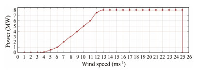
Wind resource characteristic analysis was performed using the wind turbine model Aerodyne SCD 8.0/168 (ASCD-8). This model was selected to analyze the height-dependent wind resource characteristics. The basic characteristics of ASCD-8 are summarized in Table 1, and Fig.1 plots the power curve. Note that the hub height of this model is site-specific. Considering the prospective trend of increasing the wind turbine size in the future, hub heights of 60, 80, 100, 120, 140, 160, 180, and 200 m were specified for ASCD-8.
|
|
Table 1 Basic characteristics of ASCD-8 |
|
Fig. 1 Power curve of ASCD-8. |
The WPD at height Hh is considered the main factor for wind resource characteristic analysis and is given by
| $ WP{D_{{H_h}}} = \frac{1}{2}{\rho _{{H_h}}}V_{{H_h}}^3, $ | (30) |
where
| $ {V_1} = \frac{{{V_{{\text{cut - in}}}}}}{{{{\left({{H_h}/H} \right)}^E}}}, $ | (31) |
| $ {V_2} = \frac{{{V_{{\text{cut - out}}}}}}{{{{\left({{H_h}/H} \right)}^E}}} . $ | (32) |
Previous works (Liang et al., 2020; Wen et al., 2021; Yang et al., 2023) have modeled wind speeds at various hub heights individually to determine the height-dependent WPD. However, in this study, the improved WPD at any arbitrary Hh can be acquired using the established mixture bivariate statistical models:
| $\begin{array}{l} WP{D_{{H_h}}} = \\ \;\;\frac{1}{2}\int_0^\infty {\int_{{V_1}}^{{V_2}} {{\rho _{{H_h}}}{{\left[ {{V_{{H_0}}}{{\left({\frac{{{H_h}}}{{{H_0}}}} \right)}^E}} \right]}^3}{f_{XY}}({V_{{H_0}}}, E)\text{d}{V_{{H_0}}}} } \text{d}E . \end{array} $ | (33) |
EP is another important factor in wind resource characteristic analysis (Lin and Dong, 2016). A higher magnitude of EP means that more wind electricity can be produced. In terms of offshore wind power projects, a precise estimation of EP is needed to ensure economic feasibility:
| $ EP = T \times {P_w}({V_{{H_h}}}), $ | (34) |
where T is the number of hours over a specified period and Pw(·) is the power curve shown in Fig.1. Using the developed mixture bivariate distribution model, Eq. (34) can be rewritten as
| $ EP = T\int_0^\infty {\int_{{V_1}}^{{V_2}} {{P_w}({V_{{H_h}}}){f_{XY}}({V_{{H_0}}}, E)} } {\text{ d}}{V_{{H_0}}}{\text{d}}E . $ | (35) |
The power curves are applicable under standard air density conditions. However, in practical applications, air density affects the wind resource evaluation and should be considered (Jung and Schindler, 2019a; Liang et al., 2020; Huang et al., 2023; Yang et al., 2023). Thus, to estimate wind speed under standard air density (Vst), it is imperative to transform wind speed under real air density
| $ {V_{st}} = {V_{{H_h}}}{\left({\frac{{{\rho _{{H_h}}}}}{{{\rho _{st}}}}} \right)^{z({V_{{H_h}}})}}, $ | (36) |
where ρst = 1.225 kg m−3 is the standard air density and
| $ z({V_{{H_h}}}) = \left\{ {\begin{array}{*{20}{c}} {\frac{1}{3}}&, &{{V_{{H_h}}} \leqslant 8} \\ {\frac{1}{3} + \frac{1}{3}\frac{{{V_{{H_h}}} - 8}}{5}}&, &{8 < {V_{{H_h}}} < 13} \\ {\frac{2}{3}}&, &{{V_{{H_h}}} \geqslant 13} \end{array}} \right. . $ | (37) |
Then, Vst can be computed by combining Eq. (36) and the power law profile method equation (Eq. (39)) (Gualtieri, 2019):
| $ {V_{st}} = {V_{{H_0}}}{\left({\frac{{{H_h}}}{{{H_0}}}} \right)^E}{\left({\frac{{{\rho _{{H_h}}}}}{{{\rho _{st}}}}} \right)^{z({V_{{H_h}}})}}, $ | (38) |
| $ {V_{{H_h}}} = {V_{{H_0}}}{\left({\frac{{{H_h}}}{{{H_0}}}} \right)^E}, $ | (39) |
where
| $ EP = T\int_{{E_{\min }}}^{{E_{\max }}} {\int_{{V_1}}^{{V_2}} {{P_w}\left[ {{V_{{H_0}}}{{\left({\frac{{{H_h}}}{{{H_0}}}} \right)}^E}{{\left({\frac{{{\rho _{{H_h}}}}}{{{\rho _{st}}}}} \right)}^{z({V_{{H_h}}})}}} \right]{f_{XY}}({V_{{H_0}}}, E)} } {\text{ d}}{V_{{H_0}}}{\text{d}}E . $ | (40) |
To calculate the annual energy production (AEP), T is defined as 365 × 24 = 8760. Meanwhile, to compute the seasonal energy production (SEP), T is defined as 8760/4 = 2190.
Moreover, in practical wind energy applications, CF is a crucial technical measure of the capacity of wind turbines to convert wind resources into electricity and is defined as the ratio of the AEP of a wind turbine to the rated power output over the span of one year (Quan and Leephakpreeda, 2015). Mathematically,
| $ CF = \frac{{AEP}}{{T \times {P_R}}}, $ | (41) |
where T = 8760.
2.3 Estimation of the Influence of Wind Shear VariationTo underscore the influence of wind shear coefficient variability on height-dependent wind resource characteristics, the percentage change in wind resource assessment factors (PC) was introduced and computed using
| $ PC = \frac{{{\eta _c} - \eta }}{\eta } \times 100\%, $ | (42) |
where η and ηc are the wind resource assessment factors for real wind shear coefficient conditions and the assumed constant wind shear coefficient condition (E = 0.11), respectively. Using the resulting marginal distribution of wind speed, the WPD at height Hh for constant wind shear conditions was calculated using
| $ WP{D_c} = \frac{1}{2}\int_{{V_1}}^{{V_2}} {{\rho _{{H_h}}}{{\left[ {{V_{{H_0}}}{{\left({\frac{{{H_h}}}{{{H_0}}}} \right)}^E}} \right]}^3}{f_X}({V_{{H_0}}})} {\text{ }}\text{d}{V_{{H_0}}} . $ | (43) |
Similarly, EP and CF for a constant wind shear condition can be derived from
| $ E{P_c} = T\int_{{V_1}}^{{V_2}} {{P_w}\left[ {{V_{{H_0}}}{{\left({\frac{{{H_h}}}{{{H_0}}}} \right)}^E}{{\left({\frac{{{\rho _{{H_h}}}}}{{{\rho _{st}}}}} \right)}^{z({V_{{H_h}}})}}} \right]{f_X}({V_{{H_0}}}){\text{ }}} {\text{d}}{V_{{H_0}}}, $ | (44) |
| $ C{F_c} = \frac{{AE{P_c}}}{{T \times {P_R}}} . $ | (45) |
Let PCWPD, PCEP, and PCCF be the percentage changes in WPD, EP, and CF, respectively. A positive PC value refers to the overestimation of these factors due to the assumption of a constant wind shear coefficient, and a negative value means underestimation.
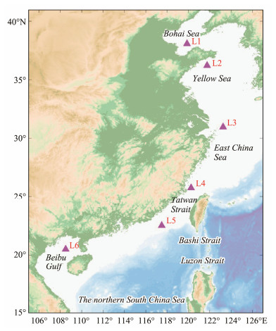
3 Data Description and AnalysisTo examine the adaptability of the designed bivariate statistical model to represent diverse wind regimes and to study the spatial characteristics of offshore wind resources, research was conducted using samples taken from six offshore wind power projects in China to represent different wind regimes in different sea areas; detailed information is presented by Yang et al. (2023). Fig.2 displays a map of the geographical distribution of the selected sites.
|
Fig. 2 Map of the adopted positions. |
The realization of a reliable and accurate wind energy evaluation can be improved by using a longer time series with high-quality data. In our work, a continuous 30-year hourly reanalysis dataset during 1993 – 2022, with the horizontal 10 m wind speed and wind shear coefficient at six positions, was taken from ERA5, which is the most contemporary reanalysis produced by the ECMWF that has undergone validation and finds widespread application in wind energy research (Soukissian et al., 2021; Patel et al., 2022; Wu et al., 2022b). The spatiotemporal resolutions for the wind parameters are 0.25˚ × 0.25˚ and 1 h (Rivas and Stoffelen, 2019; Hersbach et al., 2020).
The horizontal 10 m wind speed (V10) was calculated using
| $ {V_{10}} = \sqrt {u_{10}^2 + v_{10}^2}, $ | (46) |
where u10 and v10 are the 10 m u-component of wind and the 10 m v-component of wind, respectively, obtained from the single level product of ERA5.
The wind shear coefficient cannot be directly extracted from ERA5. The literatures (Jung and Schindler, 2017; Han et al., 2022; Debnath et al., 2023) suggested that the logarithm of both sides of the power law profile method equation (Eq. (39)) can be taken to compute the wind shear coefficient
| $ E = \frac{{\log ({V_{{H_h}}}) - \log ({V_{{H_0}}})}}{{\log ({H_h}) - \log ({H_0})}} . $ | (47) |
In this method, the wind shear coefficient can be estimated on the basis of wind speed data at two different heights and Eq. (47).
He et al. (2022) demonstrated that the power law profile method can be employed at heights less than 400 m in the atmospheric boundary layer (ABL). To acquire a more robust estimation of the wind shear coefficient, all available wind speed data with heights not greater than 400 m in the ABL were adopted in our work. The detailed procedure is presented below.
Step 1. Calculate 100 m wind speed (V100) based on the 100 m u-component and v-component of wind taken from ERA5.
Step 2. Calculate wind speeds at different pressure levels (pk (k = 1, 2, 3, 4) = 925, 950, 975, and 1000 hPa) denoted as Vk (k = 1, 2, 3, 4) using the corresponding u-component and v-component of wind taken from the pressure level products of ERA5.
Step 3. Determine the heights Hk (k = 1, 2, 3, 4) of Vk (k = 1, 2, 3, 4) using Eq. (48), which is derived from the barometric law given in Eq. (49) (Jung and Schindler, 2019a).
| $ {H_k} = \left[ {1 - {{\left({\frac{{{p_k}}}{{{p_{{H_0}}}}}} \right)}^{\frac{1}{{5.2561}}}}} \right] \times \frac{{{T_{{H_0}}}}}{{0.0065}}, {\text{ }}k = 1, 2, 3, 4, $ | (48) |
| $ {p_{{H_h}}} = {p_{{H_0}}}{\left({1 - \frac{{0.0065 \cdot \Delta h}}{{{T_{{H_0}}}}}} \right)^{5.2561}}, $ | (49) |
where
Step 4. At each hour of the investigated period, select hourly wind speed data, the heights of which are less than the ABL height (obtained from ERA5) and 400 m, from V10, V100, and Vk (k = 1, 2, 3, 4). Let Nw be the number of selected wind speed samples. If Nw is greater than 2, the least squares fitting method is employed using Eq. (47) for wind shear coefficient estimation. Otherwise, calculate this coefficient using two wind speeds with lower heights.
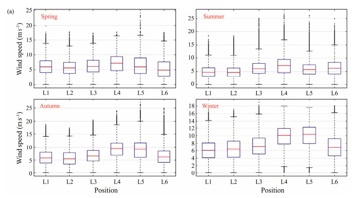
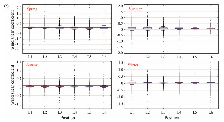
Boxplots of the total WS-SC samples at the six positions are depicted in Fig.3. Both WS-SCs show significant differences in their probabilistic distribution characteristics across various geographical positions. These variations imply that the wind resources at the six positions may differ. Specifically, position L4 records the highest wind speed median, whereas position L2 has the lowest. Position L1 has the highest wind shear coefficient median, whereas position L5 has the lowest. Note that the majority of wind shear coefficients at all chosen positions are lower than the assumed constant value (the black line in Fig.3) for offshore conditions due to different complex mechanisms (e.g., wind-wave interaction). Thus, statistical modeling of the wind shear coefficient is necessary for accurate height-dependent wind resource characteristic analysis.

|
Fig. 3 Boxplots of the total WS-SC data. |
Previous research revealed that wind energy exhibits significant seasonal variation (Shu et al., 2015; Yang et al., 2023), and the wind shear coefficient also demonstrates strong seasonality (Yan et al., 2022). Therefore, it is imperative to perform a seasonal investigation of height-dependent wind resource characteristics. The boxplots of the seasonal WS-SC samples are illustrated in Fig.4, where both variables show strong seasonal dependence. The highest wind speed median is observed in winter for all locations, whereas the lowest value is observed in spring or summer. The seasonal pattern of the wind shear coefficient is different, with the peak value in spring or summer and the minimum in autumn or winter. Season-dependent distribution characteristics emphasize the importance of seasonal analysis of wind resources.
|
Fig. 4 (a) Boxplots of seasonal wind speed. |
|
Fig. 4 (b) Boxplots of wind shear coefficient. |
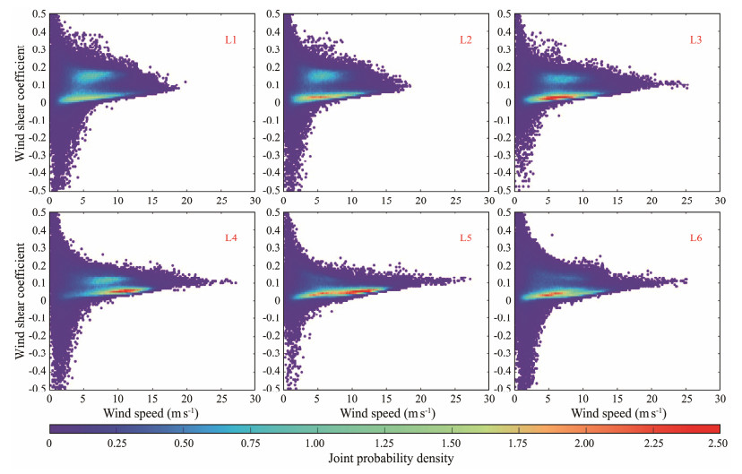
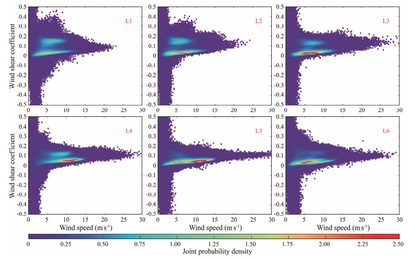
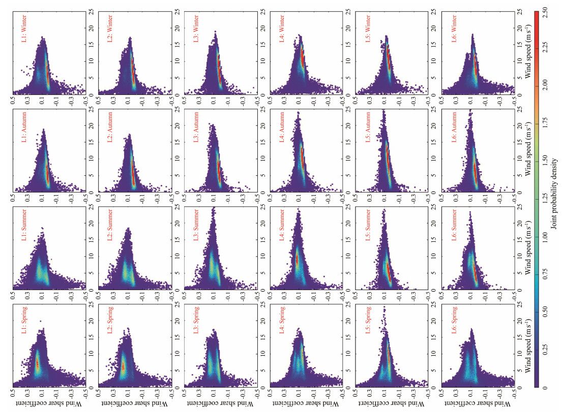
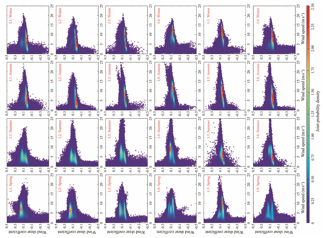
A mixture bivariate statistical model was developed in this work to capture the multimodal structures exhibited in the joint probability distribution of WS-SC. The number of components of the models for different samples was identified based on BIC. The model parameters were computed using the EM algorithm. To assess the performance of the proposed model, bivariate samples were generated. The RMSE was computed to measure the differences between the empirical data and the simulated bivariate samples, and the results are summarized in Table 2. The joint probability density plots of the WS-SC for the total samples and simulated datasets are presented in Figs.5 and 6, respectively. Similarly, Figs.7 and 8 show the joint probability density plots for seasonal data.
|
|
Table 2 Fitting accuracy for the joint statistical models of WS-SC |
|
Fig. 5 Joint probability density plots of WS-SC for the total samples. |
|
Fig. 6 Joint probability density plots of the WS-SC for the total simulated data. |
|
Fig. 7 Joint probability density plots of the WS-SC for seasonal samples. |
|
Fig. 8 Joint probability density plots of the WS-SC for seasonal simulated data. |
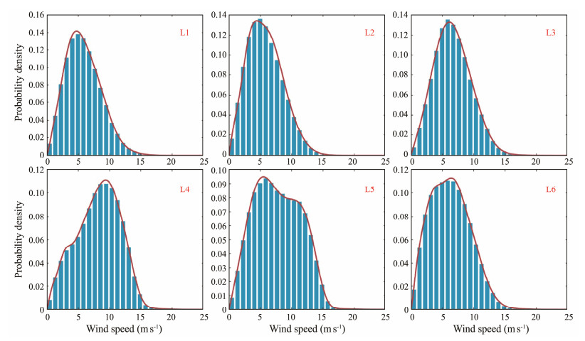
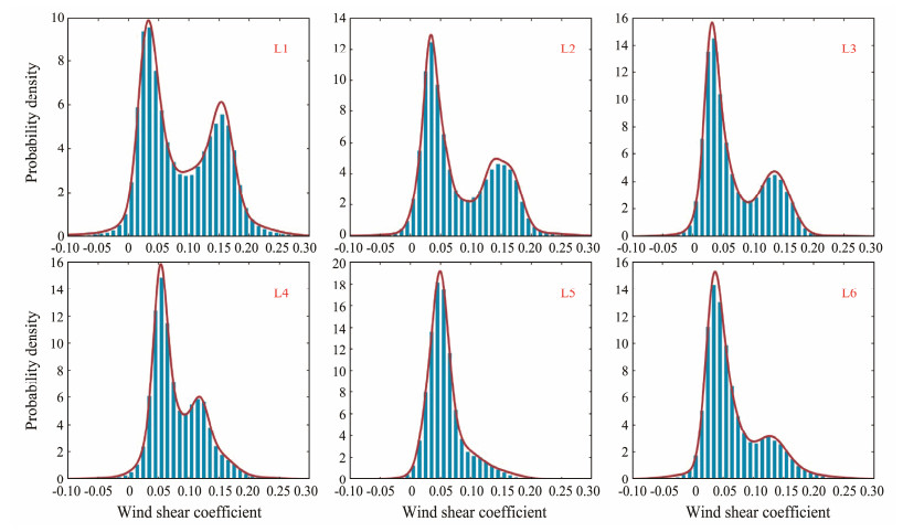
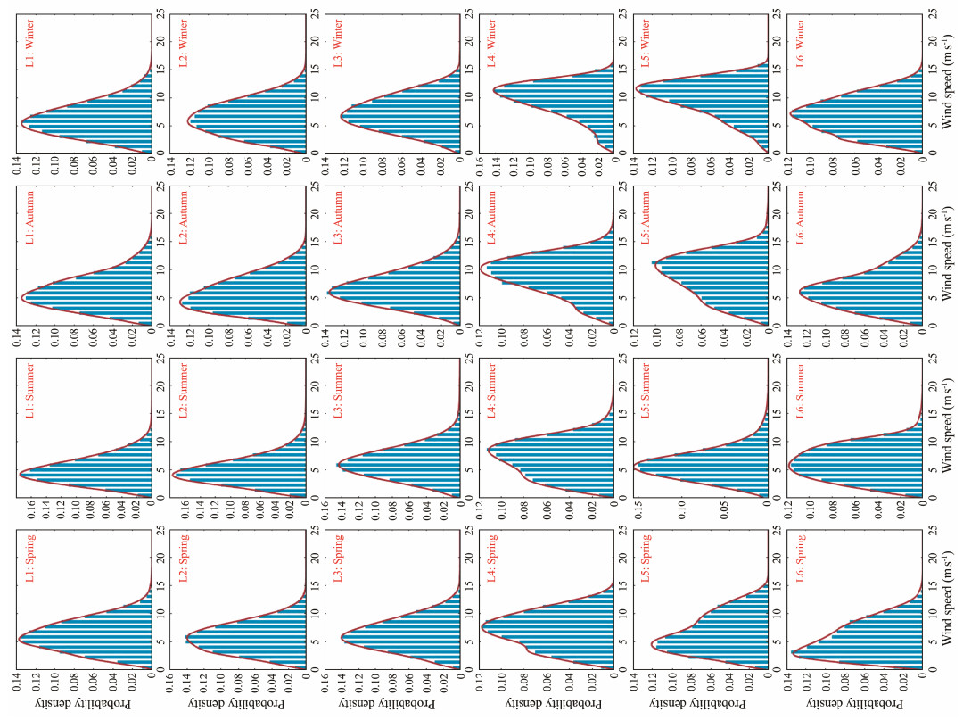
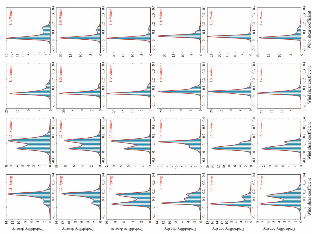
The marginal distributions of WS-SC play a critical role in practical offshore wind energy industry applications. Upon establishing the mixture bivariate statistical models, the corresponding marginal distributions for WS-SC can be derived from Eqs. (11) and (13). The marginal distributions of WS-SC for the total and seasonal samples are shown in Figs.9 − 12. To compare with the developed model, histograms of the empirical probability density distributions are also included.
|
Fig. 9 Marginal distributions of wind speed for total samples. |
|
Fig. 10 Marginal distributions of the wind shear coefficient for total samples. |
|
Fig. 11 Marginal distributions of wind speed for the seasonal samples. |
|
Fig. 12 Marginal distributions of the wind shear coefficient for seasonal samples. |
The lower RMSE values exhibit the remarkable fitting performance of the mixture bivariate model for the joint probability density distribution of WS-SC in both the total and seasonal samples. As shown in Figs.5 and 6, the peaks of the modes in the wind shear coefficient direction are widely separated, demonstrating distinct multimodal characteristics in the marginal distribution of the wind shear coefficient, as displayed in Fig.10. In contrast, there is only one hump in the probability density distributions of wind speed, as shown in Fig.9. This phenomenon occurs because the components in this direction are close to each other. The bivariate joint probability density plots of the empirical and simulated samples disclose that the developed mixture distribution model accurately captures the multimodal nature of the joint probability distribution of WS-SC.
In agreement with the distribution characteristics of WS-SC displayed in Fig.4, the probabilistic structures of these two variables show conspicuous seasonality. This phenomenon is well displayed in Figs.7 and 8. The modes of the joint distributions in the wind shear coefficient direction during autumn and winter are sufficiently near each other, resulting in unimodal marginal distributions. In contrast, the constituent components of the wind shear coefficient are far from each other, leading to the existence of two humps in the marginal distributions of this variable. The developed mixture models for seasonal data can offer adequate fitting performance for the joint distributions, further ensuring the accuracy of the seasonal wind energy characteristic analysis.
The suitability of the mixture Weibull and mixture normal distributions for WS-SC is shown in Figs.8 – 11. The marginal distributions of the wind shear coefficient for both the total and seasonal samples show multimodal characteristics that cannot be described by a single parametric model. Therefore, a linear combination of conventional distributions is needed (Huang and Dong, 2019), and the mixture normal distribution proves to be an effective fit. Note that although the probability density distributions of wind speed typically display unimodal shapes, their primary characteristics remain satisfactorily described by the mixture Weibull distribution. Thus, irrespective of whether the empirical probability density distributions are unimodal or multimodal, the mixture models can offer a suitable fit. The test statistics for the total WS-SC samples are summarized in Table 3. It can be easily observed that the established mixture univariate distributions are capable of providing outstanding fitting performances. The mixture univariate distributions for the seasonal data also show satisfactory performance, based on the results in Table 4.
|
|
Table 3 Error metrics of marginal distributions for total samples |
|
|
Table 4 Error metrics of marginal distributions for seasonal samples |
Figs.13 and 14 illustrate the height-dependent annual average WPD and seasonal average WPD, respectively. It is observed that WPD increases with increasing hub height at the investigated positions. Specifically, at L4, the annual WPD variation is greater than 200 W m−2 with changing hub height from 60 to 200 m, whereas at L6, this variation is approximately 100 W m−2. These different effects are associated with the joint distribution characteristics of WS-SC. Thus, an accurate bivariate statistical model is imperative for an accurate assessment of height-dependent WPD. The seasonal variations in WPD resulting from the changes in hub height are also significant. At L1, the seasonal WPD variation for spring can be up to 400 W m−2, whereas that for autumn and winter is only about 100 W m−2 at L1, L2, L3, and L6. These differences strongly underscore that performing a seasonal investigation of wind resource characteristics is crucial. In addition, influenced by both WS-SC, the WPD at a specific height varies significantly with space. For example, L4 and L5 have richer wind resources with annually average WPD exceeding 600 at the height of 60 m. In contrast, L1, L2, L3, and L6 have a poorer potential for offshore wind resource extraction, with an annual average WPD of less than 600 W m−2 even at the height of 200 m. As for seasonal average WPD, L1 and L2 have greater potential for wind energy in spring, whereas winter is the period with particularly abundant wind resources at L3, L4, L5, and L6.
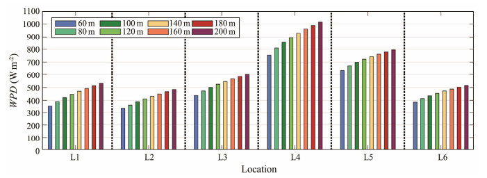
|
Fig. 13 Annual average height-dependent WPD. |
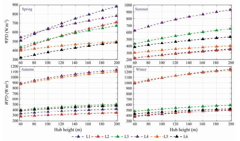
|
Fig. 14 Seasonal average height-dependent WPD. |
Figs.15 and 16 illustrate the height-dependent AEP and SEP of the selected wind turbine model. The results disclose a positive correlation between hub height and wind electricity generation, which is consistent with the WPD analysis. For instance, at L2, L3, and L4, increasing the hub height from 60 to 200 m can add approximately 5 GW h to the AEP. Similarly, peak values of variation in SEP are found in spring at L1 and L2, amounting to over 2 GW h. Notably, the rate of change in EP decreases with increasing hub height, gaining critical insights into whether the additional EP produced by a higher hub height can offset the incremental cost related to wind turbine design, manufacture, installation, and other factors, ultimately allowing cost-efficient decision-making (Jung and Schindler, 2017). The significance of this analysis is thus emphasized. Moreover, the results reveal distinct spatial and seasonal variations in the height-dependent EP. Specifically, L4 records the highest AEP, whereas L2 records the lowest. The wind turbine generates the most energy in winter at L3, L4, L5, and L6, whereas the highest SEP values are found in spring at L1 and L2. Meanwhile, the EP during summer is generally lower along the eastern coast of China.
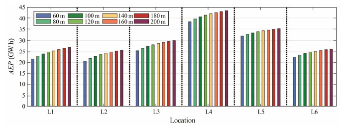
|
Fig. 15 Height-dependent AEP. |
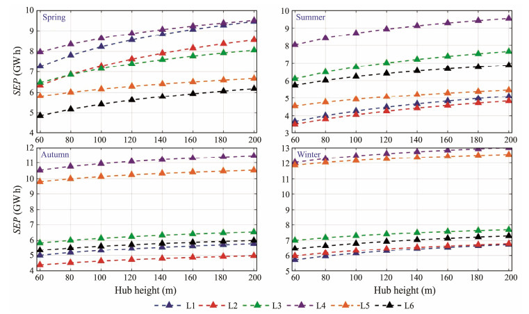
|
Fig. 16 Height-dependent SEP. |
From Eq. (41), the vertical variation and spatial distribution of the CF would coincide with those of the AEP, as presented in Table 5. Particularly, the CF increases in proportion to the hub height, with more fluctuations taking place at L2, L3, and L4, where the variation in CF results in approximately 0.08 with increasing hub height from 60 to 200 m. It is worth noting that the CF for a hub height of 200 m at L1, L2, L3, and L6 is still below 0.45, showing that the wind turbine is particularly well suited for electricity generation in these areas (de Sousa Gomes et al., 2019). Also, coinciding with the spatial distribution of the height-dependent AEP, the peak and valley values of the CF for the wind turbine are determined at L4 and L2, respectively.
|
|
Table 5 Height-dependent CF |
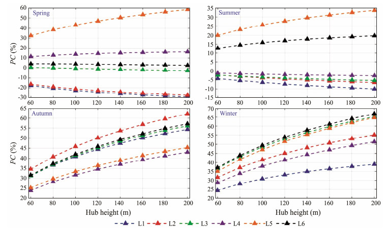
Table 6 lists the magnitudes of PCWPD for the annual average WPD, and Fig.17 presents those for the seasonal average WPD. It is shown that PCWPD generally increases with the increase in hub height for both the annual and seasonal average WPD. The median of the wind shear coefficient in Fig.3 is less than the assumed constant value, leading to negative PCWPD values, depicting an overestimation of the annual averaged WPD at all six positions. The maximum PCWPD locates at L5 with a magnitude of 52.93% at a height of 200 m due to the largest deviation between the real and assumed wind shear coefficients. L1 shows the least PCWPD, with values less than 7.5% at all studied hub heights. In addition, impacted by the seasonal variation of the wind shear coefficient, the maximum PCWPD for the seasonal average WPD is concentrated on autumn and winter. Except for the WPD of spring and summer at L1 and L2, the seasonal WPD is usually overestimated at the considered locations.
|
|
Table 6 Percentage change of annual average height-dependent WPD (%) caused by the assumed constant wind shear coefficient |
|
Fig. 17 Influence of wind shear coefficient variation on seasonal average height-dependent WPD. |
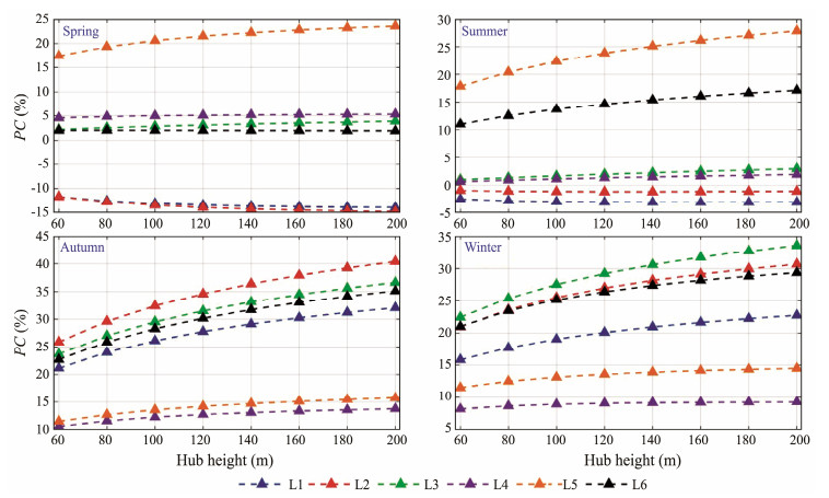
Table 7 and Fig.18 exhibit the results of PCEP for AEP and SEP, respectively. It is clear that the wind shear coefficient plays a significant role in the calculation of AEP and SEP, in particular with increasing hub heights in the future. For a particular hub height, the maximum PCEP values for the total data are observed at L6, followed by L3 or L5, whereas the minimum value is observed at L1 or L4. The PCEP values for the seasonal data are generally higher in autumn and lower in summer. Notably, a significant PCEP can seriously influence the economic feasibility assessment of offshore wind power projects in practical applications. Moreover, similar to the seasonal data results of PCWPD, the variation of the wind shear coefficient also influences SEP differently in the northern and southern regions. For example, at L1, the SEP values of spring and summer are underestimated when assuming a constant wind shear coefficient, whereas at L3, L4, L5, and L6, the SEP values of all seasons are overestimated.
|
|
Table 7 Percentage change in height-dependent AEP (%) caused by the assumed constant wind shear coefficient |
|
Fig. 18 Influence of wind shear variation on height-dependent SEP. |
In addition, based on Eqs. (44) and (47), it can be inferred that the PCCF results are identical to those of PCEP for the total data. Hence, the characteristics of the wind shear coefficient at the specified sites must be thoroughly investigated for accurate evaluation of the efficiency of the wind turbine and to determine if the selected wind turbine is a good fit for local wind conditions (Koholé et al., 2023).
5 ConclusionsIn this work, we investigated the height-dependent wind resource characteristics at six positions in the coastal sea area of China, where offshore wind farms are being planned for development. A mixture bivariate statistical model was built to model the joint distribution of WS-SC under mixed atmospheric conditions. For each component, the marginal distributions of the WS-SC were fitted using a Weibull distribution and a normal distribution, respectively, while the dependency structure was described by a Gaussian copula. The optimal number of mixture model components was determined using the BIC, and the model parameters were computed on the basis of the EM algorithm. The developed model was corroborated using both total and seasonal reanalysis data at the considered positions.
The joint probability density distributions of the WS-SC for both the total and seasonal samples at the investigated coastal positions present distinct multimodal characteristics. The developed joint statistical model can adequately capture these complex statistical patterns. Furthermore, the marginal distributions of WS-SC, whether unimodal or multimodal, can be fitted well by the proposed mixture of Weibull and normal distributions. Thus, it is suggested that mixture bivariate and univariate statistical models be utilized to model wind parameters and comprehensively evaluate wind resource potential. Also, the proposed model is an effective approach to analyzing wind resource characteristics at hub heights of 10 – 200 m. It enables the evaluation of wind resource characteristics at any arbitrary hub height without requiring measured data at a specific hub height.
The proposed model was used to assess the height-dependent wind resource characteristics at investigated positions. WPD, EP, and CF were evaluated at different hub heights, and the results demonstrate that these wind energy assessment factors increase with increasing hub height across all positions. Notably, spatial and temporal variability is found in these factors, showcasing the significance of a comprehensive spatial and seasonal investigation of height-dependent wind resources.
Moreover, the influence of wind shear coefficient variation on wind resource characteristics was quantitatively analyzed. The results demonstrated that the errors resulting from assuming a constant wind shear coefficient when calculating WPD, EP, and CF cannot be ignored, especially with the increase in hub height in the future. It was observed that these factors were overestimated at the studied positions, and the percentage change of these factors varied between the northern and southern regions. Also, the percentage change was generally higher in autumn and lower in summer for seasonal factors. Provided the potential consequences of misestimating wind resource characteristics on the economic feasibility of offshore wind power projects, proper consideration of wind shear coefficient variation and an accurate statistical model are imperative in wind energy research.
However, this work has some limitations. First, because of the lack of adequate measurements of wind speed at different heights, the wind shear coefficient was estimated using reanalysis wind speeds according to the developed procedure. In addition, only reanalysis wind speed and wind shear coefficient data at six locations along the Chinese coastline were adopted to validate the developed mixture bivariate distribution model without considering its applicability to distinct sea areas of the world. In the future, we will collect long-term wind speed observations at different heights to compute the wind shear coefficient and correct the values estimated by the reanalysis data. In addition, the general applicability of the proposed model will be shown well using more data distributed worldwide, and the influence resulting from the spatial variation of the wind shear coefficient on wind energy assessment will be further studied.
AcknowledgementsThis study was supported by the Key R & D Program of Shandong Province, China (No. 2021ZLGX04), and the National Natural Science Foundation of China (No. 52171284). The authors would like to acknowledge the ECMWF for providing the ERA5 dataset, which is available at https://www.ecmwf.int/en/forecasts/datasets/reanalysis-datasets/era5. The authors would like to acknowledge the website http://en.wind-turbine-models.com/ for providing the adopted wind turbine model.
Nomenclature
AEP, annual energy production
BIC, Bayesian information criterion
C [∙], copular function
c [∙], copula density function
CF, capacity factor
D2, squared Euclidean distance
E, wind shear coefficient
EP, energy production
FXY(·), bivariate CDF of X and Y
fXY(·), bivariate PDF of X and Y
FX(·), CDF of X
fX(·), PDF of X
FY(·), CDF of Y
fY(·), PDF of Y
Hh, hub height
KS, Kolmogorov-Smirnov distance
L(·), log-likelihood function
N, sample size
Nc, number of components in the mixture model
Nψ, size of the parameters
PC, percentage change
PCCF, percentage change in CF
PCEP, percentage change in EP
PCWPD, percentage change in WPD
PR, rated power of the wind turbine
Pw(·), power output
R, Pearson's correlation coefficient
RMSE, root-mean-square error
SEP, seasonal energy production
T, number of hours over a specified period
V, wind speed
Vcut-in, cut-in wind speed
Vcut-out, cut-out wind speed
Vst, wind speed for the standard air density condition
w, weight parameter
WPD, wind power density
x, wind speed
y, wind shear coefficient
z(·), correction variable
α, shape parameter
β, scale parameter
η, mean of y
σ, standard deviation of y
ρst, standard air density (1.225 kg m−3)
Φ(·), CDF of the standard normal distribution
γ, parameter of the Gaussian copula function
Author Contributions
All authors contributed to the study conception and design. Material preparation, data collection and analysis were performed by Zihao Yang. The draft of the manuscript was written by Zihao Yang, and all authors commented on previous versions of the manuscript. All authors read and approved the final manuscript.
Data Availability
All data generated and analyzed during this study are included in this published article and its additional files.
Declarations
Ethics Approval and Consent to Participate
This article does not contain any studies with human participants or animals performed by any of the authors.
Consent for Publication
Informed consent for publication was obtained from all participants.
Conflict of Interests
The authors declare that they have no conflict of interests.
Abu-Rayash, A., and Dincer, I., 2023. Development and assessment of an integrated wind-solar based energy system for sustainable communities. Energy Conversion and Management, 277: 116680. DOI:10.1016/j.enconman.2023.116680 (  0) 0) |
Akpinar, S., and Akpinar, E. K., 2009. Estimation of wind energy potential using finite mixture distribution models. Energy Conversion and Management, 50: 877-884. DOI:10.1016/j.enconman.2009.01.007 (  0) 0) |
Allouhi, A., Zamzoum, O., Islam, M. R., Saidur, R., Kousksou, T., Jamil, A., et al., 2017. Evaluation of wind energy potential in Morocco's coastal regions. Renewable and Sustainable Energy Reviews, 72: 311-324. DOI:10.1016/j.rser.2017.01.047 (  0) 0) |
Bai, X. Y., Jiang, H., Li, C., and Huang, L., 2020. Joint probability distribution of coastal winds and waves using a log-transformed kernel density estimation and mixed copula approach. Ocean Engineering, 216: 107937. DOI:10.1016/j.oceaneng.2020.107937 (  0) 0) |
Bilgili, M., and Alphan, H., 2022. Global growth in offshore wind turbine technology. Clean Technologies and Environmental Policy, 24: 2215-2227. DOI:10.1007/s10098-022-02314-0 (  0) 0) |
Carta, J. A., and Ramírez, P., 2007. Use of finite mixture distribution models in the analysis of wind energy in the Canarian Archipelago. Energy Conversion and Management, 48(1): 281-291. DOI:10.1016/j.enconman.2006.04.004 (  0) 0) |
Carta, J. A., Ramírez, P., and Velázquez, S., 2009. A review of wind speed probability distributions used in wind energy analysis Case studies in the Canary Islands. Renewable and Sustainable Energy Reviews, 13: 933-955. DOI:10.1016/j.rser.2008.05.005 (  0) 0) |
Chang, T. P., 2011. Estimation of wind energy potential using different probability density functions. Applied Energy, 88: 1848-1856. DOI:10.1016/j.apenergy.2010.11.010 (  0) 0) |
Cheng, Y., Chen, X., Dai, S. S., Ji, C. Y., Collu, M., Li, M. X., et al., 2022a. Wave energy extraction and hydroelastic response reduction of modular floating breakwaters as array wave energy converters integrated into a very large floating structure. Applied Energy, 306: 117953. DOI:10.1016/j.apenergy.2021.117953 (  0) 0) |
Cheng, Y., Du, W. M., Dai, S. S., Ji, C. Y., Collu, M., Cocard, M., et al., 2022b. Hydrodynamic characteristics of a hybrid oscillating water column-oscillating buoy wave energy converter integrated into a π-type floating breakwater. Renewable and Sustainable Energy Reviews, 161: 112299. DOI:10.1016/j.rser.2022.112299 (  0) 0) |
Corrigan, D., and Matthiesen, D. H., 2017. Analysis of the power law exponent applied to Lake Erie wind shear. Wind Engineering, 41(2): 103-113. DOI:10.1177/0309524X16683130 (  0) 0) |
Costoya, X., DeCastro, M., Carvalho, D., Arguilé-Pérez, B., and Gómez-Gesteira, M., 2022. Combining offshore wind and solar photovoltaic energy to stabilize energy supply under climate change scenarios: A case study on the western Iberian Peninsula. Renewable and Sustainable Energy Reviews, 157: 112037. DOI:10.1016/j.rser.2021.112037 (  0) 0) |
Dayal, K. K., Cater, J. E., Kingan, M. J., and Bellon, G. D., 2021. Wind resource assessment and energy potential of selected locations in Fiji. Renewable Energy, 172: 219-237. DOI:10.1016/j.renene.2021.03.034 (  0) 0) |
de Sousa Gomes, M. S., de Paiva, J. M. F., de Silva Moris, V. A., and Nunes, A. O., 2019. Proposal of a methodology to use offshore wind energy on the southeast coast of Brazil. Energy, 185: 327-336. DOI:10.1016/j.energy.2019.07.057 (  0) 0) |
Debnath, M., Moriarty, P., Krishnamurthy, R., Bodini, N., Newsom, R., Quon E., et al., 2023. Characterization of wind speed and directional shear at the AWAKEN field campaign site. Journal of Renewable and Sustainable Energy, 15: 033308. DOI:10.1063/5.0139737 (  0) 0) |
Dong, S., Gong, Y. J., Wang, Z. F., and Incecik, A., 2019. Wind and wave energy resources assessment around the Yangtze River Delta. Ocean Engineering, 182: 75-89. DOI:10.1016/j.oceaneng.2019.04.030 (  0) 0) |
Dong, S., Wang, N. N., Lu, H. M., and Tang, L. J., 2015. Bivariate distributions of group height and length for ocean waves using Copula methods. Coastal Engineering, 96: 49-61. DOI:10.1016/j.coastaleng.2014.11.005 (  0) 0) |
dos Santos, F. S., do Nascimento, K. K. F., da Silva Jale, J., Stosic, T., Marinho, M. H. N., and Ferreira, T. A. E., 2021. Mixture distribution and multifractal analysis applied to wind speed in the Brazilian Northeast region. Chaos, Solitons and Fractals, 144: 110651. DOI:10.1016/j.chaos.2021.110651 (  0) 0) |
Dziak, J. J., Coffman, D. L., Lanza, S. T., Li, R., and Jermiin, L. S., 2018. Sensitivity and specificity of information criteria. bioRxiv, CC BY-NC-ND 4.0, DOI: 10.1101/449751.
(  0) 0) |
Emeksiz, C., and Cetin, T., 2019. In case study: Investigation of tower shadow disturbance and wind shear variations effects on energy production, wind speed and power characteristics. Sustainable Energy Technologies and Assessments, 35: 148-159. DOI:10.1016/j.seta.2019.07.004 (  0) 0) |
Fırtın, E., Güler, Ö., and Akdağ, S. A., 2011. Investigation of wind shear coefficients and their effect on electrical energy generation. Applied Energy, 88: 4097-4105. DOI:10.1016/j.apenergy.2011.05.025 (  0) 0) |
Gong, Y. J., Wang, Z. F., Dong, S., and Zhao, Y. L., 2022. Coastal distributions of design environmental loads in typhoon-affected sea area based on the trivariate joint distribution and environmental contour method. Coastal Engineering, 178: 104221. DOI:10.1016/j.coastaleng.2022.104221 (  0) 0) |
Gualtieri, G., 2016. Atmospheric stability varying wind shear coefficients to improve wind resource extrapolation: A temporal analysis. Renewable Energy, 87: 376-390. DOI:10.1016/j.renene.2015.10.034 (  0) 0) |
Gualtieri, G., 2019. A comprehensive review on wind resource extrapolation models applied in wind energy. Renewable and Sustainable Energy Reviews, 102: 215-233. DOI:10.1016/j.rser.2018.12.015 (  0) 0) |
Guedes Soares, C., and Carvalho, A. N., 2012. Probability distributions of wave heights and periods in combined sea-states measured off the Spanish coast. Ocean Engineering, 52: 13-21. DOI:10.1016/j.oceaneng.2012.06.007 (  0) 0) |
Gupta, M. R., and Chen, Y., 2011. Theory and use of the EM algorithm. Foundations and Trends in Signal Processing, 4(3): 223-296. (  0) 0) |
Han, Q. K., Wang, T. Y., and Chu, F. L., 2022. Nonparametric copula modelling of wind speed-wind shear for the assessment of height-dependent wind energy in China. Renewable and Sustainable Energy Reviews, 161: 112319. DOI:10.1016/j.rser.2022.112319 (  0) 0) |
He, J. Y., Chan, P. W., Li, Q. S., and Lee, C. W., 2022. Characterizing coastal wind energy resources based on sodar and microwave radiometer observations. Renewable and Sustainable Energy Reviews, 163: 112498. DOI:10.1016/j.rser.2022.112498 (  0) 0) |
Hersbach, H., Bell, B., Berrisfor, P., and Hirahara, S., 2020. The ERA5 global reanalysis. Quarterly Journal of the Royal Meteorological Society, 146(730): 1999-2049. DOI:10.1002/qj.3803 (  0) 0) |
Hsu, S. A., Meindl, E. A., and Gilhousen, D. B., 1994. Determining the power-law wind-profile exponent under near-neutral stability conditions at sea. Journal of Applied Meteorology and Climatology, 33(6): 757-765. DOI:10.1175/1520-0450(1994)033<0757:DTPLWP>2.0.CO;2 (  0) 0) |
Huang, W. N., and Dong, S., 2019. Probability distribution of wave periods in combined sea states with finite mixture models. Applied Ocean Research, 92: 101938. DOI:10.1016/j.apor.2019.101938 (  0) 0) |
Huang, W. N., and Dong, S., 2021a. Joint distribution of significant wave height and zero-up-crossing wave period using mixture copula method. Ocean Engineering, 219: 108305. DOI:10.1016/j.oceaneng.2020.108305 (  0) 0) |
Huang, W. N., and Dong, S., 2021b. Statistical properties of group height and group length in combined sea states. Coastal Engineering, 166: 103897. DOI:10.1016/j.coastaleng.2021.103897 (  0) 0) |
Huang, W. N., Zhu, X. W., Xia, H. F., and Wu, K. J., 2023. Offshore wind energy assessment with a clustering approach to mixture model parameter estimation. Journal of Marine Science and Engineering, 11: 2060. DOI:10.3390/jmse11112060 (  0) 0) |
Irwin, J. S., 1979. A theoretical variation of the wind profile power-law exponent as a function of surface roughness and stability. Atmospheric Environment, 13(1): 191-194. DOI:10.1016/0004-6981(79)90260-9 (  0) 0) |
Jiang, D., Zhuang, D. F., Huang, Y. H., Wang, J. H., and Fu, J. Y., 2013. Evaluating the spatio-temporal variation of China's offshore wind resources based on remotely sensed wind field data. Renewable and Sustainable Energy Reviews, 24: 142-148. DOI:10.1016/j.rser.2013.03.058 (  0) 0) |
Jung, C., and Schindler, D., 2017. Development of a statistical bivariate wind speed-wind shear model (WSWS) to quantify the height-dependent wind resource. Energy Conversion and Management, 149: 303-317. DOI:10.1016/j.enconman.2017.07.033 (  0) 0) |
Jung, C., and Schindler, D., 2019a. The role of air density in wind energy assessment – A case study from Germany. Energy, 171: 385-392. DOI:10.1016/j.energy.2019.01.041 (  0) 0) |
Jung, C., and Schindler, D., 2019b. Wind speed distribution selection – A review of recent development and progress. Renewable and Sustainable Energy Reviews, 114: 109290. DOI:10.1016/j.rser.2019.109290 (  0) 0) |
Kavari, G., Tahani, M., and Mirhosseini, M., 2019. Wind shear effect on aerodynamic performance and energy production of horizontal axis wind turbines with developing blade element momentum theory. Journal of Cleaner Production, 219: 368-376. DOI:10.1016/j.jclepro.2019.02.073 (  0) 0) |
Kim, D. Y., Kim, Y. E., and Kim, B. S., 2021. Changes in wind turbine power characteristics and annual energy production due to atmospheric stability, turbulence intensity, and wind shear. Energy, 214: 119051. DOI:10.1016/j.energy.2020.119051 (  0) 0) |
Koholé, Y. W., Fohagui, F. C. V., Hermann, R., Djiela, T., and Tchuen, G., 2023. Wind energy potential assessment for co-generation of electricity and hydrogen in the far north region of Cameroon. Energy Conversion and Management, 279: 116765. DOI:10.1016/j.enconman.2023.116765 (  0) 0) |
Kollu, R., Rayapudi, S. R., Narasimham, S., and Pakkurthi, K. M., 2012. Mixture probability distribution functions to model wind speed distributions. International Journal of Energy and Environmental Engineering, 3: 27. DOI:10.1186/2251-6832-3-27 (  0) 0) |
Kruyt, B., Lehning, M., and Kahl, A., 2017. Potential contributions of wind power to a stable and highly renewable Swiss power supply. Applied Energy, 192: 1-11. DOI:10.1016/j.apenergy.2017.01.085 (  0) 0) |
Langodan, S., Viswanadhapalli, Y., Dasari, H. P., Knio, O., and Hoteit, I., 2016. A high-resolution assessment of wind and wave energy potentials in the Red Sea. Applied Energy, 181: 244-255. DOI:10.1016/j.apenergy.2016.08.076 (  0) 0) |
Li, J. L., Wang, X. F., and Yu, X., 2018. Use of spatio-temporal calibrated wind shear model to improve accuracy of wind resource assessment. Applied Energy, 213: 469-485. DOI:10.1016/j.apenergy.2018.01.063 (  0) 0) |
Li, J. X., Pan, S. Q., Chen, Y. P., Yao, Y., and Xu, C. H., 2022. Assessment of combined wind and wave energy in the tropical cyclone affected region: An application in China seas. Energy, 260: 125020. DOI:10.1016/j.energy.2022.125020 (  0) 0) |
Li, Q. W., Wang, J. Z., and Zhang, H. P., 2021. Comparison of the goodness-of-fit of intelligent-optimized wind speed distributions and calculation in high-altitude wind-energy potential assessment. Energy Conversion and Management, 247: 114737. DOI:10.1016/j.enconman.2021.114737 (  0) 0) |
Liang, Y. S., Ji, X. D., Wu, C. B., He, J. J., and Qin, Z. H., 2020. Estimation of the influences of air density on wind energy assessment: A case study from China. Energy Conversion and Management, 224: 113371. DOI:10.1016/j.enconman.2020.113371 (  0) 0) |
Liao, Z. K., Huang, W. N., Dong, S., and Li, H. J., 2022. Modelling trivariate distribution of directional ocean data in the Barents Sea seasonal ice zone. Ocean Engineering, 260: 111745. DOI:10.1016/j.oceaneng.2022.111745 (  0) 0) |
Lin, Y. F., and Dong, S., 2016. Assessment of seasonal wind energy at Zhifudao observation station based on joint wind speed and wind direction. Proceedings of the ASME 2016 35th International Conference on Ocean, Offshore and Arctic Engineering. Busan, South Korea, 1-10.
(  0) 0) |
Lin, Y. F., Dong, S., and Tao, S. S., 2020. Modelling long-term joint distribution of significant wave height and mean zero-crossing wave period using a copula mixture. Ocean Engineering, 197: 106856. DOI:10.1016/j.oceaneng.2019.106856 (  0) 0) |
Lucas, C., and Guedes Soares, C., 2015. Bivariate distributions of significant wave height and mean wave period of combined sea states. Ocean Engineering, 106: 341-353. DOI:10.1016/j.oceaneng.2015.07.010 (  0) 0) |
Mahmoodi, K., Ghassemi, H., and Razminia, A., 2020. Wind energy potential assessment in the Persian Gulf: A spatial and temporal analysis. Ocean Engineering, 216: 107674. DOI:10.1016/j.oceaneng.2020.107674 (  0) 0) |
Martinez, A., and Iglesias, G., 2022. Climate change impacts on wind energy resources in North America based on the CMIP6 projections. Science of the Total Environment, 806: 150580. DOI:10.1016/j.scitotenv.2021.150580 (  0) 0) |
Nie, B. C., and Li, J. C., 2018. Technical potential assessment of offshore wind energy over shallow continent shelf along China coast. Renewable Energy, 128: 391-399. DOI:10.1016/j.renene.2018.05.081 (  0) 0) |
Patel, R. P., Nagababu, G., Kachhwaha, S. S., and Arun Kumar Surisetty, V. V., 2022. A revised offshore wind resource assessment and site selection along the Indian coast using ERA5 near-hub-height wind products. Ocean Engineering, 254: 111341. DOI:10.1016/j.oceaneng.2022.111341 (  0) 0) |
Quan, T., and Leephakpreeda, T., 2015. Assessment of wind energy potential for selecting wind turbines: An application to Thailand. Sustainable Energy Technologies and Assessments, 11: 17-26. DOI:10.1016/j.seta.2015.05.002 (  0) 0) |
Ray, M. L., Rogers, A. L., and McGowan, J. G., 2006. Analysis of wind shear models and trends in different terrains. American Wind Energy Association (AWEA) Wind Power 2005 Conference. Denver, Colorado: 4-7. (  0) 0) |
Rehman, S., and Al-Abbadi, N. M., 2005. Wind shear coefficients and their effect on energy production. Energy Conversion and Management, 46: 2578-2591. DOI:10.1016/j.enconman.2004.12.005 (  0) 0) |
Rehman, S., and Al-Abbadi, N. M., 2007. Wind shear coefficients and energy yield for Dhahran, Saudi Arabia. Renewable Energy, 32: 738-749. DOI:10.1016/j.renene.2006.03.014 (  0) 0) |
Rivas, M. B., and Stoffelen, A., 2019. Characterizing ERA-interim and ERA5 surface wind biases using ASCAT. Ocean Science Discussions, 15: 831-852. DOI:10.5194/os-15-831-2019 (  0) 0) |
Shu, Z. R., Li, Q. S., and Chan, P. W., 2015. Investigation of offshore wind energy potential in Hong Kong based on Weibull distribution function. Applied Energy, 156: 362-373. DOI:10.1016/j.apenergy.2015.07.027 (  0) 0) |
Sklar, A., 1959. Fonctions de Repartition a n Dimensions et Leurs Marges. Publications de l'Institut de Statistique de l'Université de Paris, Paris, 229-231 (in French).
(  0) 0) |
Song, Y. P., Chen, J. B., Sørensen, J. D., and Li, J., 2022. Multi-parameter full probabilistic modelling of long-term joint wind-wave actions using multi-source data and applications to fatigue analysis of floating offshore wind turbines. Ocean Engineering, 247: 110676. DOI:10.1016/j.oceaneng.2022.110676 (  0) 0) |
Soukissian, T. H., Karathanasi, F. E., and Zaragkas, D. K., 2021. Exploiting offshore wind and solar resources in the Mediterranean using ERA5 reanalysis data. Energy Conversion and Management, 237: 114092. DOI:10.1016/j.enconman.2021.114092 (  0) 0) |
Svenningsen, L., 2010. Power curve air density correction and other power curve options in WindPRO. http://www.emd.dk/files/windpro/WindPRO_Power_Curve_Options.pdf.
(  0) 0) |
Tambke, J., Claveri, L., Bye, J. A. T., Poppinga, C., Lange, B., von Bremen, L., et al., 2005. Marine meteorology for Multi-Mega-Watt turbines. Proceedings of Copenhagen Offshore Wind. Copenhagen, Denmark: 1-10. (  0) 0) |
Vanem, E., 2016. Joint statistical models for significant wave height and wave period in a changing climate. Marine Structures, 49: 180-205. DOI:10.1016/j.marstruc.2016.06.001 (  0) 0) |
Wang, Q., Luo, K., Wu, C. L., Mu, Y. F., Tan, J. Y., and Fan, J. R., 2022a. Diurnal impact of atmospheric stability on inter-farm wake and power generation efficiency at neighboring onshore wind farms in complex terrain. Energy Conversion and Management, 267: 115897. DOI:10.1016/j.enconman.2022.115897 (  0) 0) |
Wang, Q., Luo, K., Wu, C. L., Zhu, Z. F., and Fan, J. R., 2022b. Mesoscale simulations of a real onshore wind power base in complex terrain: Wind farm wake behavior and power production. Energy, 241: 122873. DOI:10.1016/j.energy.2021.122873 (  0) 0) |
Wen, Y., Kamranzad, B., and Lin, P. Z., 2021. Assessment of long-term offshore wind energy potential in the south and southeast coasts of China based on a 55-year dataset. Energy, 224: 120225. DOI:10.1016/j.energy.2021.120225 (  0) 0) |
Wen, Y., Kamranzad, B., and Lin, P. Z., 2022. Joint exploitation potential of offshore wind and wave energy along the south and southeast coasts of China. Energy, 249: 123710. DOI:10.1016/j.energy.2022.123710 (  0) 0) |
Werapun, W., Tirawanichakul, Y., and Waewsak, J., 2017. Wind shear coefficients and their effect on energy production. Energy Procedia, 138: 1061-1066. DOI:10.1016/j.egypro.2017.10.111 (  0) 0) |
Wu, C. L., Wang, Q., Luo, K., and Fan, J. R., 2022a. Mesoscale impact of the sea surface on the performance of offshore wind farms. Journal of Cleaner Production, 372: 133741. DOI:10.1016/j.jclepro.2022.133741 (  0) 0) |
Wu, H., Yu, H. M., Fang, Y. Z., Zhou, Q. W., Zhuo, F. X., and Ryan, M. K., 2021. Assessment of the tidal current energy resources and the hydrodynamic impacts of energy extraction at the PuHu Channel in Zhoushan Archipelago, China. Journal of Ocean University of China, 20(3): 478-488. DOI:10.1007/s11802-021-4767-3 (  0) 0) |
Wu, S. M., Liu, J. L., Zhang, G., Han, B., Wu, R. H., and Chen, D. K., 2022b. Evaluation of NCEP-CFSv2, ERA5, and CCMP wind datasets against buoy observations over Zhejiang nearshore waters. Ocean Engineering, 259: 111832. DOI:10.1016/j.oceaneng.2022.111832 (  0) 0) |
Yan, B. W., Li, Q. S., Chan, P. W., He, Y. C., and Shu, Z. R., 2022. Characterising wind shear exponents in the offshore area using Lidar measurements. Applied Ocean Research, 127: 103293. DOI:10.1016/j.apor.2022.103293 (  0) 0) |
Yang, S. B., Xi, L. T., Li, X. F., and Zheng, C. W., 2021. Temporal and spatial characteristics of wave energy resources in Sri Lankan waters over the past 30 years. Journal of Ocean University of China, 20(3): 489-500. DOI:10.1007/s11802-021-4512-y (  0) 0) |
Yang, Z. H., Huang, W. N., Dong, S., and Li, H. J., 2023. Mixture bivariate distribution of wind speed and air density for wind energy assessment. Energy Conversion and Management, 276: 116540. DOI:10.1016/j.enconman.2022.116540 (  0) 0) |
Zhai, J. J., Yin, Q. L., and Dong, S., 2021. Co-occurrence probability of typhoon surges affecting multiple estuaries in the northern coastal region of Taiwan. Regional Studies in Marine Science, 42: 101582. DOI:10.1016/j.rsma.2020.101582 (  0) 0) |
Zheng, C. W., Pan, J., and Li, J. X., 2013. Assessing the China Sea wind energy and wave energy resources from 1988 to 2009. Ocean Engineering, 65: 39-48. DOI:10.1016/j.oceaneng.2013.03.006 (  0) 0) |
Zheng, C. W., Xiao, Z. N., Peng, Y. H., Li, C. Y., and Du, Z. B., 2018. Rezoning global offshore wind energy resources. Renewable Energy, 129: 1-11. DOI:10.1016/j.renene.2018.05.090 (  0) 0) |
Zhuo, C., Guo, J. H., Li, W., Zhang, F., Xiao, C., and Pan, Z. G., 2022. Changes in wind energy potential over China using a regional climate model ensemble. Renewable and Sustainable Energy Reviews, 159: 112219. DOI:10.1016/j.rser.2022.112219 (  0) 0) |
 2025, Vol. 24


