1 Introduction

The acoustic properties of seafloor sediments, including sound velocity and attenuation coefficient, are essential parameters that define the seafloor boundary in the marine sound field (Chaytor et al., 2023) and marine geological field (Guo et al., 2023; Liu et al., 2023). These parameters play a crucial role in various applications such as marine sound field prediction, underwater target detection, and submarine engineering investigation. Sound velocity and attenuation coefficients are fundamental parameters in marine acoustics and marine geology. They are typically determined through in-situ measurements (Zhu et al., 2017; Wang et al., 2023), sampling measurement (Li et al., 2021) or acoustic inversion techniques (Zhang et al., 2022). Seafloor sediment is commonly viewed as a two-phase solidliquid medium, influenced by the characteristics of sediment particles, pore water, and particle framework. Therefore, the acoustic properties of seafloor sediment are closely tied to the physical properties of the sediment. Developing a geo-acoustic model based on physical properties is crucial for predicting the acoustic properties of sediments in unexplored regions.

Constructing theoretical models of acoustic wave propagation in sediment is one of the main means to predict the acoustic properties of sediment. Previous studies have proposed some theoretical models, including the Biot-Stoll (Stoll, 2002), grain shearing (GS, Buckingham, 2000), and Card-House models (Ballard et al., 2014). However, these models require numerous microphysical parameters that are challenging to measure directly and must be estimated. As a result, these models have limitations in predicting sediment acoustic properties accurately (Jackson and Richardson, 2007). To address this issue, researchers often develop empirical regression equations using measured acoustic and physical characteristic data to establish relationships between acoustic properties (mainly sound velocity) and physical properties, like density, porosity, and mean particle size (Neto et al., 2013; Hou et al., 2015, 2023; Kim et al., 2018). Several studies have produced empirical regression equations, but their effectiveness varies, and they may have limitations in predicting acoustic properties accurately due to large errors in prediction. For instance, the formula proposed by Hamilton and Bachman (1982) often overpredicts sound velocity values compared to actual measurements.

Studies on the correlation between attenuation and physical properties in relation to the sound velocity of sediments are limited. The scarcity of measured data poses a challenge in establishing the necessary equations. Hamilton (1972) and Richardson and Briggs (2004) have discussed the relationship between attenuation and physical properties, with the latter providing precise fitting equations for in-situ acoustic attenuation. Wang et al. (2023) have also presented regression equations for in-situ attenuation based on data from the East China Sea. However, there is a lack of reports on attenuation prediction methods in other studies. It is noted that the correlation between acoustic attenuation coefficient and physical properties is weaker than that between sound velocity and physical properties, hindering effective sediment attenuation prediction. Therefore, the development of new technologies for creating attenuation prediction models based on physical properties is necessary.

The conventional method for estimating acoustic attenuation coefficients requires a considerable amount of attenuation data across various frequencies for fitting purposes. The limited availability of measured data continues to pose a challenge in establishing these equations. Furthermore, this method only offers acoustic attenuation coefficients for specific frequencies and does not distinguish between sedimentary acoustic attenuation at the same frequency.

In recent years, machine learning has been increasingly recognized for its significant advantages in data analysis. Several studies have suggested applying machine learning techniques to develop prediction models for sediment acoustic properties, such as sound velocity and acoustic attenuation coefficients. For instance, Hou et al. (2019) and Wang et al. (2019) utilized the random forest algorithm in machine learning to forecast sound velocity by considering parameters like porosity, particle size, water content, and wet density of sediments. Their results showed higher prediction accuracy compared to traditional empirical equations, highlighting the potential of machine learning in sedimentary acoustics.

This study aims to establish a prediction method for in-situ acoustic attenuation coefficients using machine learning technology based on particle size parameters obtained from sampling. The effectiveness of this prediction method will be evaluated by compared it with historical data to enhance the prediction system for acoustic properties of seafloor sediments.

2 Materials and Methods 2.1 In-situ Measurement

The data for this study were collected during the 2021 East China Sea spring and autumn research cruises funded by the National Natural Science Foundation of China (Cruise No. NORC2021-02 + NORC2021-301). The research data mainly include in-situ acoustic attenuation coefficients of seafloor sediments at 52 stations and particle size parameters of sediment core samples.

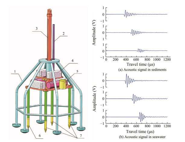
The acoustic properties of seafloor sediments are measured using ballast acoustic in-situ measurement technology (Wang et al., 2018; Li et al., 2019). This technology enables the in-situ determination of sound velocity and attenuation coefficient in 80 cm of sediment on the seafloor. The measurements are conducted using a main frequency of 30 kHz and a sampling rate of 10 MHz. The acoustic signal emitted by the transmitting transducer is captured by three receiving transducers after traversing through the sediment. To minimize measurement error and approach the true value, three channels are employed to measure and derive three distinct acoustic attenuation coefficients. Fig.1 illustrates the three-channel acoustic signal obtained through in-situ measurement. Analysis of the waveforms reveals that as the receiving distance increases, the acoustic travel time shows a nearly linearly rise, accompanied by a gradual decrease in acoustic wave amplitude. Comparing sediments of different coarseness using identical transmitting and receiving parameters, it is evident that the acoustic signal passing through coarse sediment exhibits more pronounced energy attenuation compared to fine sediment.

By using the travel time difference and amplitude difference of the three-channel received signal, the acoustic attenuation coefficient can be calculated:

$ {\alpha _p} = \frac{{20}}{l} \times \lg \frac{{{A_w}}}{{{A_p}}}, $

(1)

where α_p is the sediment acoustic attenuation coefficient, expressed in dB m⁻¹; l is the distance from the transmitting transducer to the 3 receiving transducers, expressed in m; A_p and A_w are the peak amplitudes of sediment and seawater signals collected in the same channel, respectively. The acoustic signal of three channels is obtained. Three acoustic attenuation coefficients are calculated according to the Eq. (1), and then the average value is taken as the acoustic attenuation value of the station.

2.2 Machine Learning Algorithm

The regression algorithm in machine learning is a class of algorithm used to predict the values of continuous variables. These algorithms work by modeling the relationship between input variables (independent variables) and output variables (dependent variables).

2.2.1 Random forest (RF)

The Random forest algorithm is a parallel integrated algorithm that comprises decision trees and falls under the Bagging type (Breiman, 2001). By aggregating multiple weak classifiers, the final outcome can be determined through voting or averaging, leading to high accuracy, generalization performance, and good stability. The outstanding performance of RF is primarily attributed to the incorporation of 'random' and 'forest', which offer resistance to overfitting and enhanced accuracy, respectively.

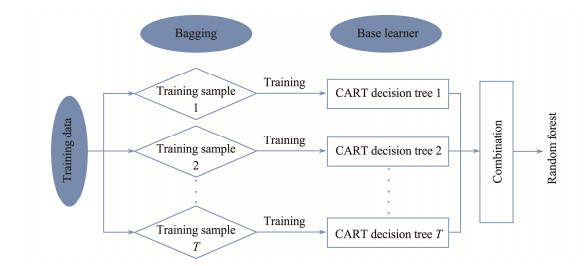
The specific operational process is outlined as follows (refer to Fig.2): initially, a dataset with m samples is considered. A sample is randomly selected for the sampling set, and then returned to the original dataset, permitting the possibility of being chosen again in the next sampling. This procedure is known as Bootstrap Sampling or Bagging. The aforementioned sampling process can be iterated T times to generate T sampling sets, each containing m training samples. A base learner is then constructed for each sample collection training, and these base learners are amalgamated. In the case of RF, the base learner employed is the CART decision tree. At each node of the base decision tree, k attributes are randomly chosen from the feature attribute set of this node, and the optimal attribute is subsequently selected from the k attributes for partitioning. This high degree of randomness induces variations among the base models. Random forest trains multiple (distinct) decision trees based on multiple (distinct) sampling sets, and employs a straightforward voting or averaging approach to enhance model stability and generalization ability.

2.2.2 Support vector regression (SVR)

In the field of regression analysis, linear regression is a commonly used method that involves fitting sample data within a vector space using linear functions. However, when a sample deviates from the linear function, it is important to assess the associated loss. Support vector regression (SVR) is a machine learning algorithm intro duced by Smola and Schölkopf (2004) to address this issue in regression analysis. The goal of SVR is to find anoptimal hyperplane that separates the dataset into distinct groups by maximizing the distance between samples on either side of the hyperplane to predict the target variable. Unlike traditional linear regression, SVR utilizes kernel functions to transform data into higher-dimensional spaces, thereby enhancing the robustness of linear regression. The key principles of SVR include data preprocessing, kernel selection, loss function optimization, and determination of hyperplane solution, all aimed at mapping data to higher-dimensional spaces and finding an optimal hyperplane to fit the data.

SVR can be considered as an optimization problem:

$ \min \frac{{{{(y- f(x))}^2}}}{{2{\varepsilon ^2}}} + \frac{{\sum\limits_{i-1}^n {{{({y_i}- f({x_i}))}^2}} }}{{2{\lambda ^2}}} . $

(2)

Among them, y represents the target variable value, f(x) represents the model's predicted value, x represents the input feature vector, n represents the number of sample points, and ε and λ are regularization parameters. The error function in the equation calculates the sum of squared differences between true and predicted values, while the regularization term limits model complexity to prevent overfitting. The optimization objective is to minimize the error function while meeting the constraints.

2.2.3 Convolutional neural network (CNN)

Convolutional neural network (CNN) is a prominent algorithm of deep learning, representing a type of deep-structured feedforward neural network that incorporates convolutional computation (Gu et al., 2018). Its key characteristic is the utilization of local connection weights sharing to reduce the number of parameters and computational complexity, thereby enhancing model accuracy and generalization capabilities. In the context of regression prediction with CNN, the principle is akin to categorical prediction. More precisely, CNN-based regression prediction involves moving a fixed-size window across the input data, applying trainable weight matrices to compute and aggregate the data within the window, resulting in an output feature map. Subsequently, the output feature map is processed into regression results through a fully connected layer. The formula for CNN's regression prediction operation is as follows:

$ z=\boldsymbol{f}_a\left(\boldsymbol{w}_x+b_a\right), $

(3)

where f_a represents the trainable weight matrix, w denotes the weight matrix, x represents the input data, and b_a represents the bias vector.

Pooling operation is used to downsample the convolved feature map in order to reduce its size while maintaining its main information. Common pooling methods include maximum pooling and average pooling.

The formula for pooling operation is as follows:

$ y = {f_s}({\text{pool}}(x)) . $

(4)

Among them, f_s represents the pooling function, pool denotes either max pooling or average pooling, and x represents the input data.

2.3 Feature Selection

Sediment grain size characteristics are fundamental properties of sediments, influenced by factors such as sediment provenance, topography, hydrodynamic conditions, transport distance, etc. The grain size of sediment contains valuable information regarding sediment provenance, transport path, climate environment, etc. This study utilizes grain size parameters as input characteristics to train the model of acoustic attenuation coefficient of sediments. Various sediment grain size parameters represent different particle sizes and shape characteristics. The grain size composition of sediment (sand, silt and clay content) indicates the proportion of particles in a sediment sample with varying diameters. 'Sand' refers to particles with a diameter ranging from 0.0625 – 2 mm, 'silt' refers to particles with a diameter ranging from 0.0625 – 0.0039 mm, and 'clay' refers to particles with a diameter generally smaller than 0.0039 mm. According to the Sheppard classification of clastic sediments (Shepard, 1954), the sediment type can be determined based on the grain size composition.

Mean particle size (Mz) represents the average size of all particles in a sediment sample, with the unit of φ. A larger mean particle size indicates a higher concentration of smaller particles in the sediment, potentially suggesting higher suspended particle concentrations in the water body. Median particle size (Md) denotes the particle size in the middle of the sorted array of all particles in a sediment sample. The Md can indicate the level of particle distribution concentration in the sediment. Sorting coefficient (Sc) reflects the degree of particle sorting resulting from physical or chemical processes during sedimentation. A higher sorting coefficient suggests a higher degree of particle sorting in the sedimentary material, possibly indicating more complex physical or chemical changes in the sedimentary environment.

The skewness value (Sk) represents the most frequently occurring particle size value in a sediment sample. A higher mode value indicates a prevalence of smaller particles, suggesting significant changes in the sedimentary environment. The kurtosis (Ku) refers to the least frequently occurring particle size value in a sediment sample. A higher peak value signifies larger particles being more common, indicating less significant changes in the sedimentary environment. The curvature coefficient (Cc) quantifies the degree of bending in particle contacts, with a higher value indicating irregular particle shapes, reflecting the influence of eddies and turbulence in fluid media. The non-uniformity coefficient (Cu) indicates the heterogeneity among sediment components, with a smaller value suggesting a more homogeneous distribution and providing insights into component interactions in the sedimentary environment.

The Mz or Md of the sediment is influenced by the particle size distribution of the source and the average kinetic energy of the transport medium. Coarse particle deposition is typical in high-energy environment, while fine particle deposition is common in low-energy environment. Therefore, the average or median particle size serves as a basis for classifying sediment sources. The sorting coefficient distinguishes the uniformity of sediment particle size, with a narrow range indicating good sorting. Sk can serves as an environmental indicator, often used to analyze the dynamic conditions and the physical processes of sediment. Sorting effects are linked to the properties of the transporting medium and distance of particle transport, while insights into sediment source and environmental conditions can be obtained through analysis of Mz, Md, and Sk.

2.4 Error Evaluation

In order to evaluate the precision of three models, namely random forest (RF), support vector regression (SVR), and convolutional neural network (CNN), we analyzed the errors of prediction results obtained from the training models. The predicted error is defined as the absolute error between the predicted value and the measured value. The mean squared error (MSE) is the average squared absolute error between the predicted and measured values. The mean absolute error (MAE) is the average absolute error between the predicted value and the measured value.

$ MSE = \frac{1}{{{N_\text{umber}}}}\sum\limits_{i = 0}^{{{\text{N}}_{{\text{umber}}}} -1} {{{({y_i}- {x_i})}^2}}, $

(5)

$ MAE = \frac{1}{{{N_\text{umber}}}}\sum\limits_{i = 0}^{{{\text{N}}_{{\text{umber}}}} -1} {{{\left| {{y_i}- {x_i}} \right|}^2}}, $

(6)

where N_umber is the number of training set, y_i is the predicted value, and x_i is the measured value. The root mean square error (RMSE) is the mean square root of the sum of squares of the deviations from the true value of each data point, representing the average errors.

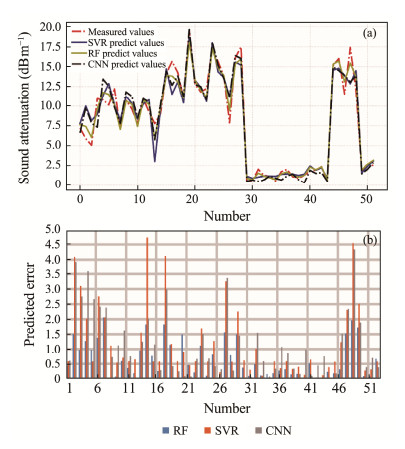
3 Results and Discussion

The training labels for supervised learning were derived from the acoustic attenuation values measured by in-situ acoustic measurement equipment. The training characteristics were determined based on particle size parameters, including sand, silt, clay contents, Mz, Md, Sk, Sc, Ku, Cc, and Cu, combined with RF, SVR, and CNN algorithms. Three prediction models were developed and their prediction errors were compared with the measured values, as presented in Table 1 and Fig.3. Among the three models, the RF model exhibited the lowest prediction error, with MSE of 0.8232, MAE of 0.6613, and RMSE of 0.9073, indicating its superior accuracy compared to the other two models.

Similarly, the comparison between the predictions of the three models and the actual measurements is depicted in Fig.3a. The results demonstrated that the predictions from the RF model closely matched the measured values, with some points overlapping. Fig.3b illustrated the discrepancy between the 52 predicted values and the actual measurements, further confirming the smaller prediction error of the RF model in comparison to the other models. It should be noted that the ranges of data used for training in this article are as follows: 0.30%<sand<89.80%, 4.10%<silt<81.50%, 1.40%<clay<54.30%, 2.17 φ<Mz<7.74 φ, 1.93 φ<Md<8.13 φ, −0.17<Skf<0.89, 0.68<Kg<3.01, 1.19<σi<2.91, 0.27<Cc<47.41, 4.64<Cu<151.20.

3.1 Feature Importance

This section aims to investigate the impact of 10 granularity parameters on a model. To achieve this objective, feature selection was conducted using the RF algorithm to determine the importance of these input parameters. The RF algorithm assesses the importance of features by analyzing the nodes of each decision tree. In each decision tree, the out-of-bag (OOB) data is utilized to calculate the outof-bag data error (errOOB1). OOB data consists of data not used in training the decision tree, which is used to assess the performance of the decision tree and determine the prediction error rate of the model, referred to as out-of-pocket data error. To assess the importance of a feature, noise interference was introduced to feature X in all samples of OOB data outside the bag randomly, and the error of data outside the bag was recalculated as errOOB2.

Assuming that there are N trees in the forest, the importance (IM) of feature X is:

$ IM = \sum\limits_{i = 1}^N {\frac{{({\text{errOOB2}} -{\text{errOOB1}})}}{N}} . $

(7)

A substantial increase in the errOOB2 value indicates a significant influence of the feature on the prediction results of the sample, indicating a relatively high level of importance.

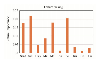
As each decision tree in a random forest is constructed based on a randomly selected subset of features, they may yield different rankings of feature importance. Nevertheless, the most important parameter features can be determined based on the feature ranking. The feature importance of the 10 granularity parameters is illustrated in Fig.4, showing that the top four features are silt, sand content, Md, and Sc.

3.2 Empirical Equations

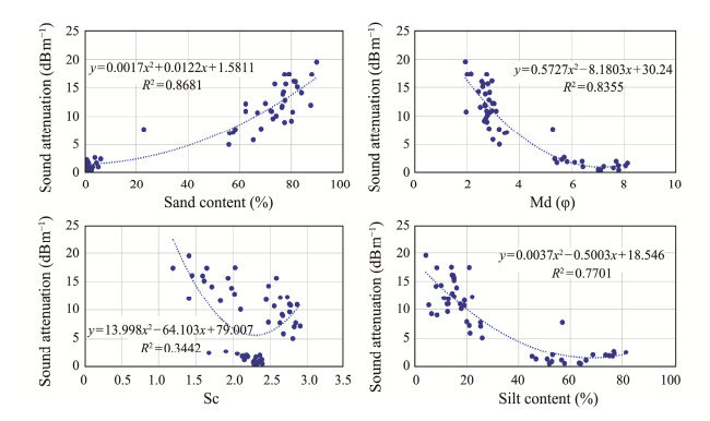
The empirical equation is a fundamental tool used to investigate the acoustic properties of sediment. Several researchers have studied the correlation between sediment physical parameters and sound velocity, resulting in the development of empirical equations for sound velocity (Hamilton, 1972; Hou et al., 2015; Kim et al., 2018; Li et al., 2021). However, developing an empirical equation for sediment acoustic attenuation has been challenging due to measurement difficulties. In this study, we utilized in-situ measurement data and feature selection analysis to establish empirical equations for acoustic attenuation based on four particle size parameters (silt, sand content, Md, and Sc). The results are presented in Fig.5, where it can be observed that the attenuation-sand equation exhibits a stronger correlation, with a coefficient of determination (R²) of 0.8681. It is noteworthy that while Sc is crucial in the RF prediction model according to feature analysis, the empirical equation indicates a weak correlation between Sc and acoustic attenuation, with an R² of only 0.3442. To assess and compare the predictive accuracy of the empirical equations and prediction models, we utilized the empirical equations to forecast data at 52 stations and compared the results with measured acoustic attenuation data (Table 1). The results indicate that the performance of these empirical equations is unsatisfactory, displaying the highest MSE, MAE, and RMSE values of 4.4571, 1.6104, and 2.1111, respectively, significantly higher than the prediction error of the prediction models. This analysis under-scores that prediction models developed using machine learning algorithms offer more precise forecasts of sediment acoustic attenuation coefficients.

3.3 Model Verification

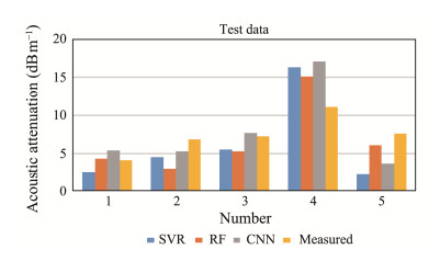
Measurements taken from the same ocean area at different periods show a high level of comparability. This study evaluated the predictive performance of three models by analyzing sandy sediment acoustic attenuation and particle size parameters from five stations in the East China Sea shelf area in 2017, using consistent measuring equipment. Despite some data collection errors, the acoustic attenuation data from 2017 and the data analyzed in this study from the same sea area demonstrated strong agreement. The particle size parameters from the five stations were inputted into the three prediction models to calculate predicted values of acoustic attenuation, which were then compared with the in-situ measurement values. The results, as depicted in Fig.6, revealed that the RF and CNN models provided prediction results that closely matched the in-situ measurement with small errors, followed by the SVR predictions. These results suggest that the three models developed in this study offer a certain degree of reliability for practical predictions.

4 Conclusions

In this study, the acoustic and physical properties of sediment samples collected in the East China Sea were analyzed. Unlike traditional regression analysis of acoustic characteristics, machine learning algorithms were employed to conduct supervised learning of acoustic attenuation coefficient and particle size parameters. Acoustic attenuation prediction models were developed based on random forest (RF), support vector regression (SVR), and convolutional neural network (CNN) algorithms.

The study compared and analyzed the prediction accuracy of the traditional empirical equation and the three machine learning algorithm models. The RF model demonstrated the lowest prediction error, with a mean squared error (MSE) of 0.8232, mean absolute error (MAE) of 0.6613, and root mean squared error (RMSE) of 0.9073, indicating superior accuracy compared to the other models and empirical equations.

Particle size parameters are essential in marine geology, and a substantial amount of particle size data has been collected from various sea regions over the years. Utilizing particle size data for predicting sediment acoustic attenuation can help overcome challenges related to the lack of input parameters for the model. A machine learning-based prediction model for acoustic attenuation offers a more effective approach for predicting acoustic attenuation in unfamiliar areas.

The main challenge we currently faced is the limited availability of precise sediment acoustic attenuation data. Both sampling and in-situ measurements require costly scientific research vessels for offshore operations, making it difficult to gather sufficient sediment acoustic attenuation data. Future research could focus on continuing to collect acoustic attenuation measurement data to expand the training dataset, as well as exploring methods to construct a more generalized prediction model using limited sample data to improve prediction accuracy.

Acknowledgements

This study was funded by the Basic Scientific Fund for National Public Research Institutes of China (No. 2022 S01), the National Natural Science Foundation of China (Nos. 42176191, 42049902, and U22A2012), the Shandong Provincial Natural Science Foundation, China (No. ZR20 22YQ40), the National Key R & D Program of China (No. 2021YFF0501202), the Southern Marine Science and Engineering Guangdong Laboratory (Zhuhai) (No. SML2023 SP232), and the Fundamental Research Funds for the Central Universities, Sun Yat-sen University (No. 241gqb006). Data acquisition and sample collections were supported by the National Natural Science Foundation of China Open Research Cruise (Cruise No. NORC2021-02 + NORC2021-301), funded by the Shiptime Sharing Project of the National Natural Science Foundation of China. This cruise was conducted onboard R/V XiangYangHong 18 by the First Institute of Oceanography, Ministry of Natural Resources, China.

Author Contributions

All authors contributed to the study conception and design. Material preparation, data collection and analysis were performed by Jingqiang Wang and Guangming Kan. The draft of the manuscript was written by Jingqiang Wang and Zhengyu Hou, the machine learning algorithms were accomplished by Zhengyu Hou and Yinglin Chen, and all authors commented on previous versions of the manuscript. All authors read and approved the final manuscript.

Data Availability

The data and references presented in this study are available from the corresponding author upon reasonable request.

Declarations

Ethics Approval and Consent to Participate

This article does not contain any studies with human participants or animals performed by any of the authors.

Consent for Publication

Informed consent for publication was obtained from all participants.

Conflict of Interests

The authors declare that they have no conflict of interests.