1 Introduction

The accurate prediction of ocean currents can not only bring valuable benefits to shipping, fishery, tourism and other fields (Hay et al., 2017), but also facilitate the accurate and timely maritime search and rescue, the exploitation of marine renewable energy, and the trajectory tracking of oil leakage and pollution. In addition, various offshore monitoring platforms and autonomous underwater vehicles will also be affected by the ocean currents when they are working (Park et al., 2020; Thippa et al., 2020; Flores et al., 2021), requiring the accurate prediction of ocean currents.

Currently, two main methods of ocean current prediction are numerical model-based and data-driven methods (Wang et al., 2022). Numerical model-based methods often use idealized assumptions and complex algorithms and are computationally time-consuming. Data-driven methods include many specific algorithms of statistics and machine learning. However, most statistical methods consider few time series features of ocean currents, and ignore the complex interrelationships between their spatial and temporal features. Because ocean currents contain abundant temporal and spatial variabilities, their spatiotemporal coupling behaviors imply the temporal correlation, spatial correlation and spatiotemporal interdependence and interactions between ocean currents in different regions at different times. In addition, deep learning networks can automatically learn and extract complex features and patterns hidden in large amount of complex data. Meanwhile, they generally have a fast and efficient real-time prediction performance, which can meet the needs of special situations, such as rapid emergency responses in case of sudden disasters and offshore engineering constructions. Therefore, constructing an efficient and trainable deep network model can help to obtain high quality and quick prediction of ocean currents. In this paper, a spatiotemporal coupled attention network is proposed to predict the ocean currents, in which 2D and 3D convolution and attention mechanisms are used to extract the spatial features and the spatiotemporal coupling features of ocean currents at the same time. Additionally, the temporal features of ocean currents are learned through the Gate Recurrent Unit (GRU) with the attention mechanism to obtain the temporal variation and interdependences between adjacent times.

2 Related Work

Ocean current prediction methods are mainly based on numerical models and data-driven methods. The numerical model generally first estimates the related meteorological or marine environmental situations in the sea area, and then infers and forecasts the ocean currents (Rui, 2019). This method includes physical models, empirical models and so on, which all rely heavily on laborious works on the model initialization and parameterization of physical processes. The numerical model is very useful for the predication of ocean currents with regular changes in motion patterns. However, it requires a lot of calculating time and increases the accumulation of errors (Jirakittayakorn et al., 2017).

Data-driven methods mainly include statistical methods and machine learning methods. Statistical methods, such as linear regression, Autoregressive Integrated Moving Average Model (ARIMA), Seasonal ARIMA (SARIMA), History Average (HA) and other time series models (Nanni et al., 2008) have also been successfully applied in the ocean current prediction. For example, a linear statistical model that took into account both the spatial and temporal correlations of data was designed and implemented to predict sea surface currents (Frolov et al., 2012). The model used empirical orthogonal function (EOF) and linear auto-regressive model to capture the spatial correlations between HF data and the temporal dynamics of EOF coefficients, respectively. Tandeo et al. (2013) proposed a regression model based on satellite surface current data and retrieved the SST gradient field to predict mesoscale surface currents. However, most methods often mainly consider the temporal dependencies of time series, but ignore the spatial dependencies between data. In addition, statistical methods cannot effectively extract complex nonlinear relationships in ocean currents.

The machine learning methods choose the relevant features of ocean currents to train a prediction model based on a large number of samples. The representative methods include Self-organizing Maps (SOM), Support Vector Machines (SVM), Support Vector Regression (SVR), Artificial Neural Network (ANN), deep learning and etc. Based on the wind data from the numerical weather prediction model (NWP), the SOM is trained to obtain the relationships between the wind and current data (Kalinić et al., 2017), and then used to estimate ocean currents. Hsiao and Hwang (2010) selected the wave height, period and ocean current velocity to predict the ocean current velocity of the port based on the modified ANN model. Their comparative experiments showed that ANN is better for predicting the ocean current velocity of the port than other statistical methods. Tettamanzi et al. (2011) proposed a data-driven evolutionary method named Covariance Matrix Adaptation (CMA) to predict the ocean currents in the Gulf of Monaco. This method was also based on the ANN model and the CMA strategy was applied to optimize the parameters of the prediction model, improving the model accuracy and interpretability. In addition, there were hybrid models combining statistical model and machine learning, such as the ARIMA-BP neural network hybrid model (Chao, 2014) and a Kalman filter based on long short-term memory (Zhang et al., 2019). However, these methods did not consider both the spatial and temporal characteristics of ocean currents. Since deep learning methods have strong feature learning abilities, they have been successfully applied in automatically extracting complex spatial and temporal features from ocean currents. Thongniran et al. (2019b) proposed an ocean current prediction model CNN_GRU that combined CNN with GRU to extract the spatial and temporal features of ocean currents respectively. On the basis of CNN_GRU, Thongniran et al. (2019a) designed and implemented the ocean surface current prediction model with the help of modern techniques such as soft attention mechanisms, transfer learning and domain knowledges. Although these works took the spatiotemporal characteristics of ocean currents into account when prediction, they extracted spatial and temporal features sequentially by different independent structures, which led to the loss of some important coupling features and limited the performance of prediction. In addition, Immas et al. (2021) realized the prediction of the velocity and direction of ocean currents based on LSTM and Transformer method, and suggested that the attention-based methods exceeded the performance of RNN in many prediction tasks. In this paper, we build a new module to extract the spatiotemporal coupling features of ocean currents synchronously, which avoids the feature separation problem caused by the asynchronous feature extraction architecture. We also design and implement the attention module to capture the spatial correlations of the predicted sea areas and the interaction of the ocean currents between different approaching times and the present prediction time.

3 Dataset and Preprocessing 3.1 Dataset

Two datasets are used in this study. One is called MediSea_Dataset, which is the data set from part of the Mediterranean Sea area, and the other is called EastSea_Dataset, which is the coastal data set of eastern China. The initial data set is in NetCDF format, and the time resolution is daily.

1) The MediSea_Dataset is provided by the European Center for Medium-term Weather Forecasts (ECMWF) and are daily gridded sea level data from global ocean satellite observations. The spatial resolution is 0.125°, and the coverage area is 29.47° – 45.16°N, 6.00°W – 36.60°E, with a total of 128 × 344 grid points. The time span is from January 1, 2016 to December 31, 2019, a total of four years. It mainly contains seven attribute fields, namely, 'time', 'latitude', 'longitude', 'Ugosa', 'Vgosa', 'Ugos', 'Vgos', which mean recording time, latitude, longitude, north component of absolute geostrophic flow, east component of absolute geostrophic flow, north component of geostrophic flow and east component of geostrophic flow.

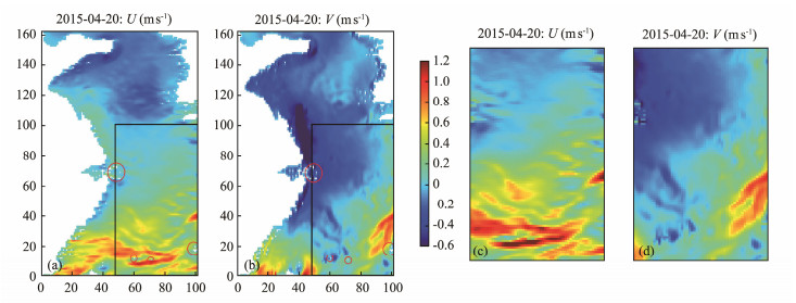
2) The original EastSea_Dataset mainly covers the coastal sea area of eastern China and is collected from the HYCOM numerical model. The spatial range of data is 25° – 38°N, 119° – 127°E, and the geospatial resolution is 0.08°, with a total of 163 × 101 grid points. The time span is from April 18, 2014 to April 18, 2018, a total of four years. It mainly contains five attribute fields, i.e., 'time', 'latitude', 'longitude', 'U', 'V'. As shown in Fig.5, the EastSea_Dataset used in this paper is only a subset of this original EastSea_Dataset, generated by intercepting operation, with a total of 100 × 55 grid points.

3.2 Data Preprocessing

1) Data removal and imputation

Firstly, we intercept the EastSea dataset into the size of 100 × 55 grid points. Then, we supplement the missing data at certain points by considering both the impact of adjacent times and adjacent regions around. The specific steps are as follows: for the missing data of edge points or edge times, the average value of the most adjacent data in space and moment is used for filling. For the missing data in the middle points or the middle times, the data of the adjacent times and the four adjacent positions in space are taken and averaged to fill the data. The black box areas in Figs.1a and 1b indicate the intercepted area of our data, and the filled results are shown in Figs.1c and 1d accordingly. In order to obtain more spatial correlation information and balance the efficiency, the dataset is further divided into several patches whose numbers are determined according to the scale of ocean currents for parallel model training. Based on many experiments, the size of the patches is finally set to 5°× 5°. There are 220 patches in total.

2) Data normalization

The data normalization ensures that different features have the same scale and eliminates the dimensional influence between features. The normalization method used in this paper is min-max normalization, which converts the sample data range into 0 – 1 by the function. This processing can not only accelerate the convergence rate of the model and reduce the training time, but also improve the accuracy of the model prediction.

3) Data partitioning

In this paper, all the dataset is randomly divided into training set and test set, accounting for 75% and 25% respectively, among which the validation dataset accounts for 12% of training dataset. Furthermore, we consider that ocean current data contain a large amount of spatiotemporal information, so we use the following two strategies to retain both spatial information and temporal information when dividing the training and test datasets to improve the prediction results.

a) Retain spatial information: When entering the spatial module, the input data containing space and time dimension are reshaped as the format of (batch_size, time-steps, width, height, channels).

b) Retain temporal information: When entering the nearest neighbor time attention module, the input data containing the time dimension are reshaped as the format (batch_ size, time-steps, channels).

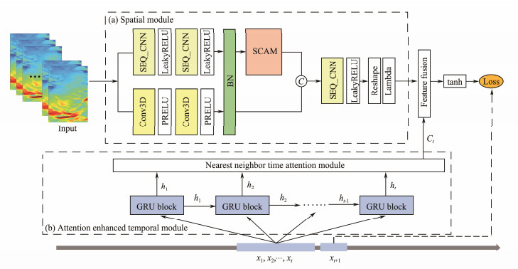
4 Methods

The temporal and spatial characteristics of ocean currents are often complex and coupled, so in this paper we design and implement a model STCANet that can extract the potential spatiotemporal coupling characteristics of ocean currents. Based on sliding window, the STCANet uses the historical time series of current velocity components U and V (as input) obtained from the previous N timesteps to predict the current velocity of the next timestep (as output). In the sensitivity analysis experiment of Section 4.5, N can be set as 7, 15, 30, 45 and 60 days, representing the time span of one week, half month, one month, one and a half month and two months respectively. The overall architecture is shown in Fig.2. By means of 2D convolution and 3D spatiotemporal convolution, a new spatial module is constructed to simultaneously extract complex spatiotemporal coupling features, in which a spatial channel attention module (SCAM) is used to obtain the correlation degree of spatial interdependencies between different sea areas. In addition, our ocean current prediction model also considers certain correlations between adjacent times. Therefore, the nearest neighbor attention module is added into GRU to extract the temporal correlation information to improve the accuracy of ocean current prediction. Finally, the spatiotemporal coupling features and the attention enhanced temporal information are fused by the feature fusion layer, and the full connection layer activated by tanh function is used to predict the ocean current at the next timestep.

4.1 Spatial Module

In order to effectively learn the behavior characteristics of ocean currents, a Spatial Module based on 2D-convolution, 3D-spatiotemporal convolution and a spatial attention mechanism is designed and implemented in this paper. The spatial module structure is shown in Fig.2a, and its design and implementation details are presented as follows.

1) Sequence convolution layer

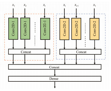
A new convolution layer structure SEQ_CNN (Fig.3) is designed and implemented to extract the global and local spatial information of ocean currents. In the SEQ_CNN structure, the global spatial feature F_global and the local spatial feature F_local are obtained by computing on the ocean current data of the same period with convolution kernels of different sizes, namely, Conv2D-1 uses kernel sizes according to local features and Conv2D-2 uses convolution kernel size of 3 for global features. Then the obtained F_global and F_local are spliced and the fused spatial feature information is activated through the dense layer.

In this Module, the feature map $ X \in {\mathbb{R}^{T \times H \times W \times C}} $ is fed into SEQ_CNN, and then after the treatment of the Leaky-RELU activation layer (Fig.2a), a higher-level feature $ {H_1} \in {\mathbb{R}^{T \times H \times W \times {C_1}}} $ will be obtained, where T, H, W represents the timesteps, height, and width of the ocean current data respectively, while C and C₁ represent the channels of ocean current components. After the second layer of SEQ_CNN and the LeakyRELU activation layer are processed and output, the higher-level spatial information $ {H_2} \in {\mathbb{R}^{T \times H \times W \times {C_1}}} $ in the predicted sea area is obtained. As shown in the green unit in Fig.2a, the BN layer transforms the input data of each hidden layer into a standard normal distribution that conforms to (0, 1), that is, the spatial information H₂ from SEQ_CNN and LeakyRELU is processed by BN to get $ {F_S} \in {\mathbb{R}^{T \times H \times W \times {C_1}}} $.

2) Spatial channel attention module

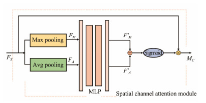
In order to better characterize the different impact of ocean currents in different input sea areas on those in the predicted sea area, spatial channel attention module (SCAM) is designed and implemented to extract the correlation information between different input sea areas and the predicted sea area. The architecture is shown in Fig.4.

The spatial feature $ {F_S} \in {\mathbb{R}^{T \times H \times W \times {C_1}}} $ is compressed in the spatial dimension by the maximum pooling layer and the average pooling layer to obtain two features $ {F_M} \in $ $ {\mathbb{R}^{T \times 1 \times 1 \times {C_1}}} $ and $ {F_A} \in {\mathbb{R}^{T \times 1 \times 1 \times {C_1}}} $. Then F_M and F_A are input into the customized multi-layer perceptron (MLP) by RELU at the same time to obtain two new outputs $ {F'_M} \in $ $ {\mathbb{R}^{T \times 1 \times 1 \times {C_1}}} $ and $ {F'_A} \in {\mathbb{R}^{T \times 1 \times 1 \times {C_1}}} $. Then F'_M and F'_A are fused to obtain the weight of spatial feature relationship of each channel by the sigmoid activation function, and the spatial correlation information $ {M_C} \in {\mathbb{R}^{T \times H \times W \times {C_1}}} $ is obtained by the weighted summation with feature F_S (Eq. (1)), so the spatial correlations between different areas around the specific ocean currents are extracted.

$ {M_C} = {F_S}\left({{\text{Sigmoid}}\left({{\text{Concat}}\left({{{F}'_M}, {{F}'_A}} \right)} \right)} \right) . $

(1)

.In addition, the feature map $ X \in {\mathbb{R}^{T \times H \times W \times C}} $ is fed into Conv3D and LeakyRELU to generate a new higher-level feature, and it is processed by BN to get $ {F_{ST}} \in $ $ {\mathbb{R}^{T \times H \times W \times {C_2}}} $. Then the F_ST and M_C are spliced and input to another SEQ_CNN layer and LeakyRELU to get F_spatial∈ $ {\mathbb{R}^{T \times H \times W \times 1}} $.

4.2 Attention Enhanced Temporal Module

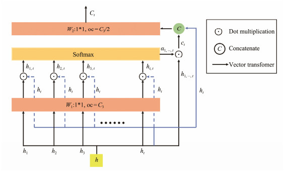
In order to better understand the temporal correlations between the historical data of ocean currents, in this paper an attention mechanism is designed and implemented to learn the nearest neighbor time correlations in ocean currents. As shown in Fig.5, the hidden state of GRU output $ h \in {\mathbb{R}^{N \times T \times {C_3}}} $ is input into a linear activation layer with the training weight of W₁ to obtain $ {H_S} \in {\mathbb{R}^{N \times T \times {C_3}}} $. Then the correlation value $ {S_t} \in {\mathbb{R}^{N \times T}} $between H_S and the hidden state h_t at the last moment is calculated. Then, the probability distribution α_i of the correlation value S_t in this period is obtained through the Softmax function (Eq. (2)). After that, α_i and the initial hidden state h are weighted and summed to calculate the context vector c_t∈ $ {\mathbb{R}^{N \times T \times {C_3}}} $ (Eq. (3)), which mainly contains the impacts of the closely adjacent times. Then hidden state h_t at the last moment and the context vector c_t are concatenated and passed into a full connection layer with a training weight of W₂ to generate the nearest neighbor time correlation information $ {C_t} \in {\mathbb{R}^{N \times T \times \frac{{{C_3}}}{2}}} $ (Eq.(4)).

$ {S_t} = h_t^Th{W_1}, $

(2)

$ {c_t} = \sum\limits_{i = 1}^t {{\alpha _i}{h_i}}, $

(3)

$ {C_t} = \tanh ({W_2}[{c_t}:{h_t}]) . $

(4)

Finally, the spatial feature F_spatial output by spatial module and the temporal feature C_t output by attention enhanced temporal module are activated by the feature fusion layer and the full connection layer, and the output feature $ {F_{t + 1}} \in {\mathbb{R}^{1 \times H \times W \times C}} $, namely, the ocean current prediction information at T + 1 is obtained.

5 Experiments 5.1 Parameter Setting and Evaluation Metrics

Based on our datasets in Section 3, all experiments in this paper are performed on an NVIDIA GeForce GTX 1080 Ti with 11 GB memory and implemented based on python 3.6 using Tensorflow as the Keras framework running at the backend. In order to compare with benchmark models, we set the same parameters for our model and the compared models as follows: batch_size is set to 300, training epoch is set to 100, hyperbolic tangent function is used as loss function, Adam is used as optimizer, and 1e-3 is used as learning rate. Additionally, for our STCANet model, the specific hyperparameters settings are fine-tuned and used for our experiment, as shown in Table1. The hyperparameters settings of benchmark models are shown in Table 2.

The ocean current prediction belongs to a regression problem. In this paper, the evaluation metrics of regression problems such as Mean Absolute Error (MAE), Root Mean Square Error (RMSE) are used for comparative analysis of the models. MAE is the mean value of absolute errors between model fitting data and original data, and can be calculated by the following formula:

$ MAE = \frac{1}{n}\sum\limits_{i = 1}^n {\left| {\mathop {{\phi _i}}\limits^ \wedge - \mathop {{\phi _i}}\limits^{} } \right|} . $

(5)

MSE refers to the mean of the sum of squares of errors between the model fitting data and the original data at the corresponding points. RMSE is the square root of MSE, which can be expressed as the following formula:

$ RMSE = {[MSE]^{\frac{1}{2}}} = {\left[ {\frac{1}{n}{{\sum\limits_{i = 1}^n {\left({\mathop {{\phi _i}}\limits^ \wedge - \mathop {{\phi _i}}\limits^{} } \right)} }^2}} \right]^{\frac{1}{2}}}, $

(6)

where $ {\hat \phi _i} $ is the predicted value, φ_i is the real value, and n refers to the number of all data points. Here, RMSE and MAE are calculated based on the predicted ocean current values of the next day and the real values in the test set from the MediSea_Dataset and EastSea_Dataset. And the lower MAE and RMSE are, the higher the accuracy of the prediction is.

5.2 Comparison with Other Prediction Models

In order to evaluate the effectiveness of our model STCA-Net, we choose benchmark data driven models of the ocean current prediction for comparison, including the following 2 types: Statistics-based time series models and deep learning models. Statistics-based time series models include Historical Average (HA) and Auto-Regressive Integrated Moving Average (ARIMA), while Deep Learning Models include MLP, CNN, LSTM, GRU, CNN_GRU (Thongniran et al., 2019b) and CNN_Att_GRU (Thongniran et al., 2019a). The prediction effects of different models on EastSea_Dataset and MediSea_Dataset are compared under the evaluation metrics of RMSE, MAE and differences. Differences refer to the gap of RMSE between different models and STCANet, which is used to measure the improvement level of our model compared with the benchmark models. The calculation formula is as follows:

$ {\text{Differences}} = \frac{{RMSE({\text{STCANet}}) - RMSE({\text{baseline}})}}{{RMSE({\text{baseline}})}} . $

(7)

The comparison results on the EastSea_Dataset and MediSea_Dataset are presented in Tables 3 and 4, respectively. On the whole, our model has achieved state-of-the-art results on both MAE and RMSE. The prediction results of U and V velocities on the EastSea_Dataset have the lowest RMSE of 0.1881, 0.1536 and MAE of 0.1234 and 0.1130. Specifically, the prediction qualities of statistical models including HA and ARIMA are significantly lower than those of deep learning models, because they are completely dependent on historical values for prediction. MLP further takes the context characteristics of ocean currents into account and achieves better prediction results than HA and ARIMA, but it does not consider the temporal and spatial characteristics of ocean currents. Although CNN can capture spatial characteristics, LSTM and GRU can capture temporal characteristics, and they achieve better prediction results than MLP, the prediction qualities of CNN, LSTM and GRU are significantly lower than those of STCANet model. Compared with the previous ocean current prediction model CNN_GRU, the prediction qualities of the proposed model in this paper for U and V are increased by 18.7% and 16.7% on EastSea_Dataset, respectively, and the RMSEs of Ugos and Vgos are both increased by 59.8% on MediSea_Dataset.

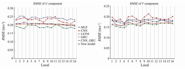
In addition, this paper also explores the prediction qualities of different models in a part of the sea areas we studied. The timestep of this experiment is set to 7, and the prediction results of U and V components in the local areas are shown in Fig.6. Among them, the horizontal axis indicates 16 patches in the study area with a grid resolution of 5° × 5°, and the vertical axis represents the RMSE between the predicted values and the real values. The smalller the RMSE is, the better the prediction accuracy is. Obviously, the prediction accuracy of our new model is better than other models.

5.3 Ablation Experiment

The ablation experiment is conducted to prove the effectiveness of the modules of spatial characteristics extraction and temporal characteristics extraction for the ocean current prediction. In order to describe the ablation experiments more conveniently, the modules with different combinations are given new names as follows.

MODULE_A: Spatial module (CNN) + temporal module (GRU);

MODULE_B: Spatial module (SEQ_CNN + SCAM) + temporal module (GRU);

MODULE_C: Spatial module (STCANet[S]) + temporal module (LSTM) + Spatial_temporal feature fusion layer;

MODULE_D: Spatial module (STCANet[S]) + temporal module (GRU) + Spatial_temporal feature fusion layer;

MODULE_E: Spatial module (STCANet[S]) + temporal module (GRU + nearest neighbor time attention module) + Spatial_ temporal feature fusion layer.

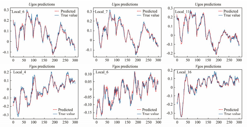
The experimental results are shown in Table 5. For MODULE_A, although the temporal and spatial characteristics for the ocean current prediction are considered based on the CNN and GRU respectively, its prediction result is not as better as that of MODULE_B. Because MODULE_ B incorporates the SEQ_CNN and SCAM modules instead of CNN, while keeping the GRU unchanged to capture temporal characteristics, it considers the influences of both the local and global spatial information on ocean current prediction. MODULE_C, MODULE_D and MODULE_E are all incorporate the same STCANet[S] and the Spatial_temporal feature fusion layer for capturing the spatial characteristics of ocean currents and fusing the spatial and temporal characteristics. The difference between MODULE_C, MODULE_D and MODULE_E is that they combine three different temporal characteristics extraction modules: LSTM, GRU and GRU + nearest neighbor time attention module, respectively. MODULE_D achieves better prediction results than MODULE_C according to the RMSE and MAE metrics. This is because GRU reduces a gated mechanism compared with LSTM, which can better realize the convergence of the model. However, MODULE_E achieved the better prediction quality than MODULE_D, which additionally incorporates the nearest neighbor time attention module for learning the influence of data at different adjacent times on the ocean current at the predicted time. The experimental results, shown in Table 5, demonstrates the effectiveness of our designed modules for improving the prediction quality of ocean currents. In addition, to further demonstrate the effectiveness of STCANet model, we visualize the predicted ocean current components in the local area based on MediSea_Dataset (Fig.7). For each prediction result diagram, the horizontal axis represents the time, and the vertical axis represents the predicted Ugos or Vgos components of ocean currents. Among them, the blue solid line represents the curves of true values, and the red dotted line represents the curves of predicted values. For different ocean current components, this paper finally selects three local regions to show the prediction results. The Ugos components are visualized in three local patches with the geographical ranges of (32.27° – 35.07°N, 16.5° – 19°E), (35.07° – 37.87°N, 16.5° – 19°E) and (35.07° – 37.87°N, 19° – 21.5°E), named as Local_6, Local_7 and Local_11 respectively, while the Vgos components are visualized in three local patches with the ranges of (37.87° – 40.67°N, 14° – 16.5°E), (32.27° – 35.07°N, 16.5° – 19°E), and (37.87° – 40.67°N, 21.5° – 24°E), named Local_4, Local_6 and Local_16. According to the prediction results shown in Fig.7, compared with Vgos, the prediction quality of Ugos is better, which are basically consistent with Table 4.

5.4 Sensitivity Analysis

In order to explore the sensitivity of our proposed method to timesteps, batch size, dataset normalization, optimizers, we carried out the sensitivity analysis from the following three aspects.

1) Timesteps and batch_size

When adjusting the hyper-parameters of the model, the first step is to explore the influence of batch_size and timesteps on the prediction results of the model. The batch_ size determines the number of training samples when the model is trained once, and the timesteps directly relates to the amount of historical information that the new model can retain. Here, the batch_size of 50, 100, 150, 200, 250 and 300 are used. The timesteps is set in accordance with multiple time scales of week, half month, whole month, one and a half month, two months.

According to the experimental results listed in Tables 6 and 7, for the U component, when the batch_size is set to 100 and the timesteps is set to 60, the prediction effect of STCANet model is the best. When the timesteps is set to 45, the performance improvement is not obvious, but the corresponding time cost will not increase significantly. Therefore, the batch_size of 100 and the timesteps of 45 are finally set to train the prediction model. For the V component, when the batch_size is 300 and the timesteps is 30, the evaluation metric RMSE and MAE of the model are the lowest with the best prediction results.

2) Dataset normalization

In this paper, min-max normalization is used to standardize our dataset, and for the global and local sea areas, global normalization and local normalization are used respectively. The global normalization is used to firstly standardize the whole dataset and then divide the dataset. The local normalization first divide the whole dataset into several data subsets according to patches and then standardize the data subset in each patch separately. In order to select the best standardization way, this paper has carried out experimental verification on MLP, CNN, LSTM, GRU, CNN_GRU, STCANet. The comparison results are shown in Table 8. According to the experimental results, the RMSE of local normalization is about 1.6% to 6.2% lower than that of global normalization.

3) Optimizers and learning rates

In order to find a better optimizer for the prediction, we compare several optimizers such as SGD, RMSProp, Adagrad, Adadelta, Adam, and Nadam. NAG and Momentum optimization are combined with SGD and other optimizers. Each optimizer uses the default parameter settings for experiments, and the prediction results of our model on the U and V components are shown in Table 9. The optimizer with the best prediction effect is Adam. When the learning rate of Adam is 0.001, the model can achieve a better prediction result.

6 Discussion 6.1 Separate or Integrated Input and Output of U and V Components

Since the two velocity components U and V of the ocean current, can be combined into one integrated variable in physics, we further carried out the current prediction experiments taking the integrated two components as the input. The MediSea_Dataset and EastSea_Dataset are the experimental data set, and timesteps = 7, future_timesetps = 1, batch_size = 100, epoch = 100. The experimental results are listed in Table 10.

It can be seen from Table 10 that when U and V components are input and output separately for the ocean current prediction, the RMSEs of the models based on both MediSea_Dataset and the EastSea_Dataset are lowest, which has the highest accuracy. When U and V components are input together, the corresponding RMSE is obviously higher, and the accuracy of predicting the integrated U and V together is slightly lower than that of predicting U and V separately. Currently, there are some researches (Thongniran et al., 2019a, 2019b) that input and predict the U and V components separately, similar to our method. However, users can also choose to input or output the two components together for prediction according to their own needs.

6.2 Seasonal and Periodic Influence

Ocean current has obvious seasonal and periodic changes over time. Therefore, in addition to consider the correlation of adjacent times, the seasonal and periodic variation characteristics of ocean currents should also be considered when prediction. Here, we compared the prediction accuracy of our model before and after the de-seasonalizing to the EastSea_Dataset based on Z-score method (as shown by the Eq. (8)).

$ {x'_i} = \frac{{{x_i} - \mu }}{{\sigma t}}, $

(8)

where x_i represents the original daily ocean current data, μ and σ_t represent the mean and standard deviation of the daily ocean current components calculated by x_i, respectively. The prediction results are shown in Table 11.

It can be seen from Table 11 that after de-seasonalizing, the prediction accuracies of the ocean current components based on MediSea_Dataset and EastSea_Dataset are obviously higher than those without de-seasonalizing. Therefore, considering the seasonality variation characteristics of ocean current data will help to improve the prediction accuracy of the models.

6.3 3D Current Prediction

In this paper, we consider the 2D spatio-temporal coupling characteristics of ocean currents to predict the surface currents, and the experiments show that the fusion of multidimensional characteristics including time and 2D space information simultinously is effective. As we all know, the marine current is 3D in space, and the deeper waters also has significant impact on the surface currents. Therefore, we will extend the model to a 3D space to further improve the quality of the model in the future. For lack of reliable underwater dataset, currently, we only implemented the prediction of ocean surface currents. However, we can extend our model to 3D current predicition by easily adding a depth dimension to the input. Moreover, the current is usually complex and affected by many other factors like wind and air sea interactions such as heat flux, which have direct impacts on the movement of ocean currents. Therefore, we will consider more influencing factors in our model to predict the status of ocean currents more accurately.

7 Conclusions

In this paper, we propose a novel deep network prediction model STCANet that can extract the spatiotemporal coupling characteristics of ocean currents. Firstly, we design a spatial and temporal feature extraction module to simultaneously extract the complex spatiotemporal coupling features in ocean currents, and solve the separation problem of spatial and temporal features in previous models. Secondly, the spatial channel attention mechanism is used to capture the spatial correlations between different areas at a certain time. In addition, we use the GRU module to obtain the temporal patterns implied in ocean current data, and design the nearest neighbor time attention module to extract the temporal correlations among the adjacent time series data. Finally, a series of experiments are carried out on the MediSea_Dataset and EastSea_Dataset, and compared with the benchmark models such as HA, ARIMA, LSTM, GRU, CNN_GRU under the evaluation metrics of MAE and RMSE. The results show that our STCANet model has the higher prediction accuracy than other models. In the future, we will consider more influence factors of ocean currents, involve the physical characteristics of ocean current itself and try the prediction of deep ocean currents. In addition, the ocean current is easily affected by external environmental factors such as wind, seawater density, temperature, etc. Therefore, we will try to introduce these external factors into the model and design the reasonable module to learn their correlations with ocean currents for further improving the accuracy of prediction.

Acknowledgements

The authors would like to thank the financial support from the National Key Research and Development Program of China (Nos. 2020YFE0201200, 2019YFC1509100), the partial support by the Youth Program of Natural Science Foundation of China (No. 41706010), and the Fundamental Research Funds for the Central Universities (No. 202264002).