1 Introduction

The Southern Ocean (SO) is an essential part of global wind-driven and thermohaline circulation, with complex dynamic connections to the atmosphere and the deeper ocean (Thompson et al., 2011). It is critical in the global energy and carbon cycle and thus regulates global climate and bioecological processes (Sarmiento et al., 2004; Marshall and Speer, 2012). For instance, the SO has absorbed most of the heat (about 75%) and anthropogenic carbon (about 50%) in recent decades due to its broad low temperature and large upwelling system (Fig.1a), significantly delaying the increase in global mean surface temperature (Sabine et al., 2004; Quéré et al., 2007; Kuhlbrodt and Gregory, 2012; Frölicher et al., 2015; Roemmich et al., 2015). Coupled climate models are a primary tool to understand the SO states and their role in global climate change. Accurate simulation of the SO climate in the historical period is one of the key parameters for evaluation of the performance of state-of-art climate models. However, climate models suffer from substantial systematic biases in simulation of the SO sea surface temperature (SST), with broad striking warm biases in most regions of the SO that contrast the cold biases in the Northern Hemisphere (Fig.1b) (Gupta et al., 2009; Meijers, 2013; Wang et al., 2014; Hyder et al., 2018; Purich et al., 2021; Farneti et al., 2022; Luo et al., 2023).

Earlier generations of climate models have common deficiencies such as coarse grids, imperfect parameterization schemes, and incomplete physical process characterization, which inevitably lead to biases in reproducing the observed climate. With the continuous development of models in recent decades, more refined model grids, more reasonable parameterization schemes, and biochemical cycles have been introduced in the state-of-the-art climate models (Eyring et al., 2016). Current climate models have taken a leap forward and become an important tool for people to understand the climate system. However, the SO SST warm biases persist in the coupled models participating in phases 5 and 6 of Coupled Model Intercomparison Project (CMIP5 and CMIP6) (Meijers, 2013; Wang et al., 2014; Sallée et al., 2015; Hyder et al., 2018; Luo et al., 2023). This issue challenges the reliability of future projections by climate models (Kajtar et al., 2021) and thus needs evaluations on the characteristics of the SO SST bias and investigations on the possible origins of the SO SST biases (He and Soden, 2016; Collins et al., 2018).

In CMIP5 models, Hyder et al. (2018) suggest that the prominent warm biases in CMIP models are anchored to the regions at 40˚ – 60˚S with excessively high surface net heat flux in the atmospheric component-alone simulations. The reason that the SST biases are not anchored by the sea surface net heat flux of CMIP itself is that there is significant flux compensation from the ocean-atmosphere coupling processes in the CMIP simulations. The overly high sea surface net heat flux is further suggested to primarily result from excessive shortwave radiation arising from deficiencies in cloud parameterization schemes, including a lack of reflective supercooled liquid water in parameterization schemes (Mann et al., 2010; Bellouin et al., 2013; Furtado et al., 2016; Williams et al., 2017). The SO SST biases may also be associated with the mixing efficiency of the upper ocean (Belcher et al., 2012; Fan and Griffies, 2014). In the climate model GFDL-CM2M designed by the Geophysical Fluid Dynamics Laboratory (Dunne et al., 2012), both the improved stratified Langmuir turbulence mixing scheme (Smyth et al., 2002) and the surface nonbreaking wave mixing scheme (Qiao et al., 2004; Chen et al., 2020) can effectively lower the simulated bias of upper ocean temperature and heat content in the Southern Hemisphere (SH) Ocean. Zhang et al. (2023) proposed that the cloud and noncloud components of the surface radiation both contribute to the formation of the SO SST biases. However, the quantitative contributions from different local atmospheric and oceanic processes on the formation of SO SST biases based on the mixed layer (ML) heat budget have not been studied; some studies focused on the atmospheric processes but ignored the oceanic conditions, such as those by Hyder et al. (2018) and Zhang et al. (2023).

In addition, the number of models employed in most of the earlier studies on the SO SST biases is relatively small, and there are highly similar biases in homological models developing from the same community (Wang et al., 2014; Hyder et al., 2018; Luo et al., 2023), which obscures the systematical evaluation and investigation on the underlying processes of the long-lasting SO SST biases in the CMIP5 and CMIP6 models. Moreover, the differences in local SST biases between models are highly associated with the differences in global-mean systematic biases due to substantial differences in parameterization schemes of atmospheric cloud and convection and ocean mixing. However, the effect of homological models and global-mean biases on the evaluation of the SO local SST biases has not been examined.

Thus, this work presents an analysis of a large ensemble of CMIP5 and CMIP6 models and assesses the change in SO SST simulations from CMIP5 to CMIP6 models, accompanied by homological models and removing the effect of global-mean SST biases to underscore the local changes. The underlying local processes generating the SO SST biases are measured by the ML heat budget, with an emphasis on the zonal-mean results as the SO climatology SST is primarily characterized as zonal bands and the zonal-mean simplifies the underlying processes involved in the formation of the SST biases. This paper is structured as follows. Section 2 describes the data and method. Section 3 shows the results. Section 4 highlights the summary and discussion.

2 Data and Methods 2.1 Observation and Reanalysis Data

To assess the model-simulated SO SST climatology during the historical period by CMIP models, the Extended Reconstruction SST version 5 (ERSSTv5, Huang et al., 2017) dataset is utilized. The ERSSTv5 integrates the global monthly mean SST from the International Comprehensive Ocean-Atmosphere Data Set, the National Centers for Environmental Prediction in the United States observed global monthly average SST on site, and the Hadley Center Sea Ice and SST (HadISST) from the UK Met Office. The surface wind from the Cross-Calibrated Multi-Platform (CCMP, Atlas et al., 2011; Mears et al., 2022) is also employed.

2.2 CMIP Models and Outputs

The outputs of historical simulations from CMIP5 (1850 – 2005, Taylor et al., 2012) and CMIP6 (1850 – 2014, Eyring et al., 2016) models are utilized, such as the monthly mean SST, surface heat flux, surface wind, ML depth (MLD), potential temperature, salinity, and seawater velocity (Table 1). Only one member (such as r1i1p1 in CMIP5 and r1i1p1f1 in CMIP6) of each model is chosen to ensure equal contribution from different models. Moreover, the outputs from the Atmospheric Model Intercomparison Project (AMIP) corresponding to CMIP are utilized to separate the intrinsic biases in the atmospheric component of the coupled models (Ceppi et al., 2012; Long et al., 2020). The AMIP simulations are forced by observed monthly mean SST and sea ice (Webb et al., 2017). The study period for observation and model simulations of CMIP and AMIP is 1979 – 2005.

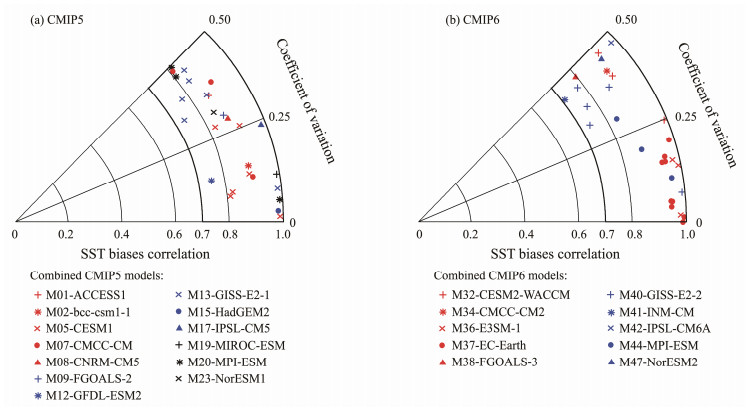
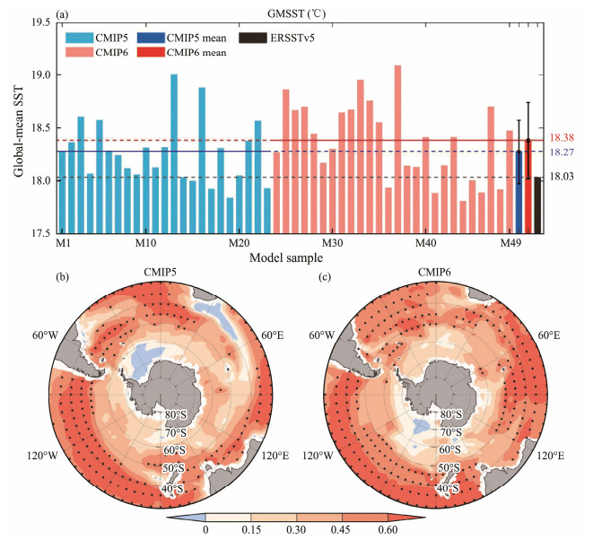
Some models taking part in CMIP are designed from the same community and share highly similar SO SST biases in both magnitude and spatial pattern, i.e., homological models. Fig.2 illustrates that any two models of the selected homological model ensemble generally display the SO SST biases with high spatial correlation coefficients greater than 0.7 and similar magnitudes, with a small coefficient of variation (C_v = std/mean, where std refers to the standard deviation across members in the ensemble and mean refers to the ensemble-mean value) below 0.5. Note that any two members from the chosen homological model ensemble are estimated as one point in Fig.2; the number of the points is calculated using C_n² (where n denotes the number of members). Thus, there is only one point for M01 because it has only two members (ACCEESS1.0 and ACCESS1.3) but 6 points for M13 because it has four members (GISS-E2-H, GISS-E2-H-CC, GISS-E2-R, and GISS-E2-R-CC). If all homological models are employed, it may result in an overweight or misinterpretation of the model biases in these communities when performing multimodel ensemble-mean (MME) and intermodel correlation analyses. Thus, we combine the homological models into one model sample. Through this processing, the original 85 model samples are decreased to 49 model samples (Table 1), with 23 from CMIP5 and 26 from CMIP6. The model dependence is thus substantially increased and can more reasonably be utilized for the performance evaluation of models across communities and trace the origins of the SO SST biases. Moreover, Fig.3a exhibits that the climatology of global-mean SST (GMSST) during 1979 – 2005 is substantially different across models due to systematical intermodel differences in the dynamical core, mixing parameterization, cloud physical processes, etc. To eliminate the effect of global-mean biases, we subtract the GMSST bias from the local SST bias at each grid for each model.

2.3 Methods 2.3.1 Intermodel empirical orthogonal function analysis

In climate studies, empirical orthogonal function (EOF) analysis is often used to contract the dominant spatial modes of the variability in climate metrics and how the modes evolve with time. To comprehend the intermodel variability of the SST biases in CMIP models, intermodel EOF analysis is used to understand the underlying physical processes modulating the differences in biases across models. Compared with the traditional EOF analysis based on spatiotemporal anomaly fields, intermodel EOF analysis is performed based on spatial model bias fields, i.e., the time series is replaced by the intermodel series. The spatial pattern of the intermodel EOF shows the mode of the intermodel variability, while the principal components denote the differences in the corresponding spatial pattern across models.

2.3.2 ML heat budget

Changes in SST are primarily determined by the ML heat budget (Morioka et al., 2010; Xie et al., 2010; Schneider and Fan, 2012), which considers the effect of oceanic conditions such as MLD and horizontal and vertical advection on SST change. For instance, at the same amount of ML heat input, the deep ML temperature increases at a smaller magnitude compared with the shallow ML temperature. The ML heat budget equation is:

$ \frac{\partial T}{\partial t}=\frac{Q_{\mathrm{net}}}{\rho_0 C_p h}-\vec{u} \cdot \nabla T-\frac{w_e\left(T-T_d\right)}{h}+r e s, $

(1)

where ∂T/∂t refers to the derivative of SST over time, T and T_d refer to the SST and seawater temperature at the bottom of the ML, respectively, Q refers to the actual heat flux entering the ML (net heat flux is denoted as Q_net), $ \vec{u}$ and w_e refer to the horizontal current and vertical velocity at the base of the MLD, respectively, ρ₀ refers to the seawater density (1027 kg m⁻³), C_p refers to the specific heat capacity of seawater (4096 J (kg℃)⁻¹), h is MLD, and res refers to the residual term. In climatology, there is merely a balance between the terms on the right hand of Eq. (1) as the temporal variation can be ignored (Xie et al., 2010; Schneider et al., 2012; Long et al., 2014):

$ 0=\frac{Q_{\mathrm{net}}}{\rho C_p h}-\vec{u} \cdot \nabla T-\frac{w_e\left(T-T_d\right)}{h}+r e s . $

(2)

Eq. (2) implies that there is a substantial offset between the surface heat adjustments and ocean dynamical adjustment to maintain the SST climatology. From the energy balance view, models with a high climatological SST need an additional heat source from either surface heat flux or ocean advection compared with models with a low climatological SST. Thus, models with a warm SST bias, i.e., higher SST climatology than that in observation, require an extra source of heat from the term on the right hand compared with the observation. This gives a clue to explore the origin of the SST biases by the ML heat budget. However, given that there is large uncertainty in the surface heat flux and ocean currents from reanalysis products, we compute the differences between top and bottom models instead to examine the contributions of different processes on the bias formation. Subtracting the same term in Eq. (2) between the top and bottom models,

$ 0=\Delta\left(\frac{Q}{\rho_0 C_p h}\right)-\Delta(\vec{u} \cdot \nabla T)-\Delta\left(\frac{w_e\left(T-T_d\right)}{h}\right)+r e s . $

(3)

The first item on the right of Eq. (3) refers to the surface heat flux effect, while the second and third terms refer to the effects of horizontal and vertical advection. For the surface heat flux term, it can be further decomposed as follows:

$ \Delta \left({\frac{Q}{{{\rho _0}{C_p}h}}} \right) = \frac{{\Delta Q}}{{{\rho _0}{C_p}h}} - \frac{Q}{{{\rho _0}{C_p}h}} \cdot \frac{{\Delta h}}{h} + res, $

(4)

where ∆Q is the difference in Q between the two models, and ∆h is the difference in MLD. On the right of Eq. (4), the first and second terms refer to the effect of the difference in Q and MLD, respectively, and the third term is a residual. For the ocean advection heat transport term, it can be expressed as follows:

$ \Delta (\vec u \cdot \nabla T) = \Delta \vec u \cdot \nabla T + \vec u \cdot \Delta (\nabla T) + \Delta \vec u \cdot \Delta (\nabla T). $

(5)

The first and second terms on the right of Eq. (5) exhibit the effects of differences in ocean currents and ocean temperature, respectively, and the third term indicates the nonlinear effect of the decomposition. These diagnostic decompositions can aid in understanding the specific contributions of atmospheric and oceanic processes in producing the SO SST biases.

3 Results 3.1 Comparison of the SO SST Biases in CMIP5 and CMIP6 Models

Fig.3a illustrates that the climatology of GMSST during 1979 – 2005 is substantially different across models. The MME GMSST is 18.27℃ in CMIP5, with an intermodel std of 0.29℃, and 18.39℃ in CMIP6, with an intermodel std of 0.37℃. The MME GMSST of CMIP6 models is 0.12℃ warmer than that of CMIP5 but with increased intermodel spread, possibly attributed to an increased climate sensitivity from substantially updated cloud parameterization in some current climate models (Zelinka et al., 2020). Furthermore, there is a significant intermodel correlation between the SO local SST biases and the GMSST, particularly at the latitude north of 50˚S (Figs.3b, 3c). This implies that models with a higher GMSST tend to show a warmer SO SST. Thus, the intermodel differences in global-mean systematical biases would impact the estimation of the regional SST biases, which should be eliminated when assessing the differences between CMIP5 and CMIP6 and examining the local origins of the SO SST biases in MME and intermodel analyses.

Given that the homological models and GMSST biases are common issues in multimodel evaluation, which have not been well addressed in most of the previous studies, we first explore the respective and joint effects of the two issues on the model bias evaluation between CMIP5 and CMIP6 (Table 2). Without considering the two issues, the SO warm biases at 70˚ – 30˚S would increase from 0.36℃ in CMIP5 to 0.54℃ in CMIP6 (an increase of 50%) and the intermodel std is decreased from 0.83℃ in CMIP5 to 0.64℃ in CMIP6 (a decrease of 23%). This is also similar for the low- (45˚ – 30˚S) and high-latitude (70˚ – 45˚S) of the SO and consistent with Zhang et al. (2023), who used 28 CMIP5 models and 33 CMIP6 models to assess the SO SST. The differences in MME value and the intermodel std would decrease even if only one of the two issues is addressed. For instance, from CMIP5 to CMIP6, the MME 70˚ – 30˚S warm bias is reduced from 0.41℃ to 0.43℃ after the combination of homological models alone and from 0.4℃ to 0.43℃ if only the GMSST differences are eliminated. If the two issues are both addressed, the MME 70˚ – 30˚S warm bias is decreased from 0.38℃ in CMIP5 to 0.28℃ in CMIP6 (a decrease of 26%) compared with the results without addressing the two issues. It is worth noting that the warm SST biases still increase at the low latitude after the two issues are addressed despite the model consistency being increased from CMIP5 to CMIP6. This is because, in the CMIP5 ensemble, some models show prominent cold biases at the low latitude that largely weaken the warm biases in MME, while there are consistent warm biases in the CMIP6 ensemble, which is discussed here. The results imply that the effect of homological models and GMSST differences should be considered in multimodel analyses of the SO SST biases, and the following analyses are performed with the homological models combined and the GMSST biases removed.

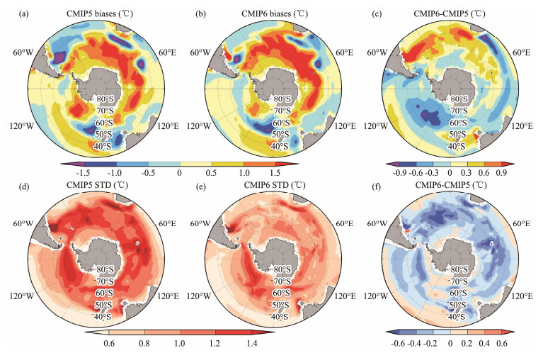
Fig.4 presents the MME biases in the combined 23 CMIP5 models and 26 CMIP6 models after the removal of the intermodel differences of GMSST biases. In CMIP5, prominent and broad warm biases are observed at the high-latitude SO, especially at 60˚ – 40˚S and in the Atlantic and Indian sectors. In the Pacific sector, the simulated SST is generally slightly warmer than the observation (Fig.4a). The cold SST biases distribute scatteredly at the low latitude of the Atlantic Ocean, the southeast of the Cape of Good Hope, and the southeast of Australia. As a consequence, the CMIP5 MME is characterized as warm biases in the SO to the first order. For CMIP6, the spatial pattern of SST biases highly mimics that of CMIP5 but with a reduced magnitude in some regions (Fig.4b). The decreased SST in CMIP6 is primarily contributed by the reduced warm biases in the Indian and Pacific sectors and improved cold biases between 60˚ – 50˚S and 160˚W – 180˚ (Fig.4c).

The intermodel std is comparable to or even greater than the MME biases in magnitude (Figs.4d, 4e), demonstrating a large intermodel spread. The area-mean intermodel std of the SO SST biases is 0.74℃ in CMIP5 models and reduced to 0.58℃ in CMIP6 (Figs.4e, 4f, Table 2). Indeed, the decreased intermodel std is also apparent in the results without considering the effect of homological models and GMSST differences, indicating a substantial increase in the consistency of the simulation of the SO SST in CMIP6 models.

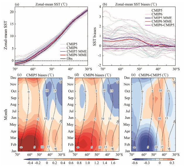
In general, the SO SST exhibits consistent warm biases south of 50˚S while the cold biases mainly appear north of 50˚S despite the large zonal variations (Fig.4). For simplicity and to extract the major feature of intermodel differences in the SO biases, we hereafter focus on the characteristics and origins of the zonal-mean SO SST biases. The CMIP5 and CMIP6 models show warm SO biases at all latitudes, particularly south of 50˚S, but with large intermodel spread (Figs.5a, 5b). At the low-latitude SO, the zonal-mean SST biases are between −1℃ and 1℃ and largely compensate for each other across models, leaving weak MME warm biases north of 45˚S. In general, the MME SO SST biases are closer to the observation in CMIP6 than CMIP5 south of 50˚S.

In the SO, substantial seasonality is observed in the SST biases (shading in Figs.5c, 5d) following the seasonal variations in climatology SST (Figs.5c, 5d). The seasonal varied SST is primarily a consequence of the seasonal differences in atmospheric conditions, such as surface wind, heat flux, and freshwater flux, and oceanic conditions, such as MLD. In both CMIP5 and CMIP6, the high-latitude warm biases are much larger in austral summertime (December – May) than in wintertime (June – November). At low latitudes, minor warm biases appear in summertime while cold biases emerge in wintertime; the seasonal cancellation of the warm and cold biases causes reduced annual-mean MME biases. From CMIP5 to CMIP6, the reduction in annual mean warm biases primarily takes place in summertime at 70˚ – 45˚S (Fig.5e) when the warm biases are the largest, with a maximal reduction of 0.6℃. In general, the CMIP6 models show enhancement in simulating the SO SST regarding the reduced seasonal warm biases and increased model consistency compared with the CMIP5 models, which may be attributed to the enhanced surface heat flux from shortwave radiation (not shown). However, the SO SST biases are still robust across models and thus warrant further investigation of their causes in both CMIP5 and CMIP6. Provided large uncertainty and mismatch in atmospheric and oceanic variables from reanalysis datasets, we thus trace the origins of the SO SST biases by intermodel analyses as the atmospheric and oceanic variables are physically constrained among models.

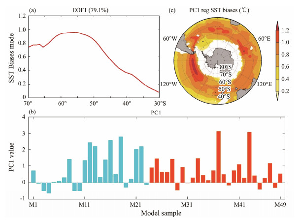
3.2 Dominant Mode of the Intermodel Variations in the SO SST Biases

The comparison between CMIP5 and CMIP6 models discloses that despite displaying some enhancement, the SO SST biases are still prominent in CMIP6 models, implying that the main origins of the biases persist from CMIP5 to CMIP6. We thus perform intermodel EOF analysis on the zonal-mean SST biases based on 49 combined model samples from both CMIP5 and CMIP6 to extract the dominant pattern of the intermodel spread in the SO SST biases. The first EOF mode (EOF1) explains 79.1% of the intermodel variance (Fig.6a), which is dominant and warrants in-depth investigation. The EOF1 shows warm biases that are large at the high latitude but weak at the low latitude, which aligns with the MME pattern. The principal component of the EOF1 (PC1, Fig.6b) is positive for most models but negative in a few models. Indeed, the intermodel correlation between PC1 and the SO area-mean biases is high (0.92). The regression of the intermodel SST biases against PC1 also exhibits an overall warm bias pattern (Fig.6c), with high values over regions of large intermodel std. Thus, EOF1 and PC1 can well capture the basic MME structure and differences in the SO SST biases across models on the zonal-mean scale.

The PC1 shows that 12 model samples have an overall weak cold SST bias pattern. We select the six model samples with the largest negative PC values, i.e., CanESM2, CanESM5, MRI-ESM2-0, FIO-ESM, BNU-ESM, and FGOALS-2, which are denoted as the Cold-model ensemble. The six model samples with the largest positive PC values are denoted as the Warm-model ensemble, i.e., MIROC6, EC-Earth3, MIROC5, inmcm4, GFDL-ESM2, and GISS-E2-1. It is worth noting that the Cold-model ensemble has much smaller PC values than the Warm-model ensemble, which can provide near-observation reference in the investigation of the underlying physical processes for the SO SST biases according to differences between the Warm-model and Cold-model ensembles.

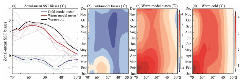
The composite zonal-mean SST biases show an opposite meridional structure between Warm-model and Cold-model ensembles (Fig.7a). The cold biases are generally weaker than −1℃ at all latitudes and relatively large around 50˚ – 35˚S in the Cold-model ensemble. Conversely, the Warm-model ensemble displays significant warm biases at all latitudes, especially south of 40˚S. For the Cold-model ensemble, the intermodel spread is large at the low latitude but weak at the high latitude, but for the Warm-model ensemble, it is large at all latitudes. Also, the seasonal evolutions of the composite warm and cold biases in the two ensembles (Figs.7b, 7c) are similar to those of the 49 model samples (Figs.5a, 5b), with warm biases during summertime and cold biases or weak warm biases during wintertime. The differences between the Warm-model and Cold-model ensembles are very similar to the results of the Warm-model ensemble on annual and seasonal scales (Fig.7), laying the foundation for the subsequent analyses based on their difference rather than comparing the model outputs with uncertain reanalysis products.

3.3 Diagnostic Contributions of Different Processes Causing the SO SST Biases

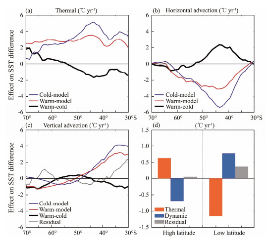
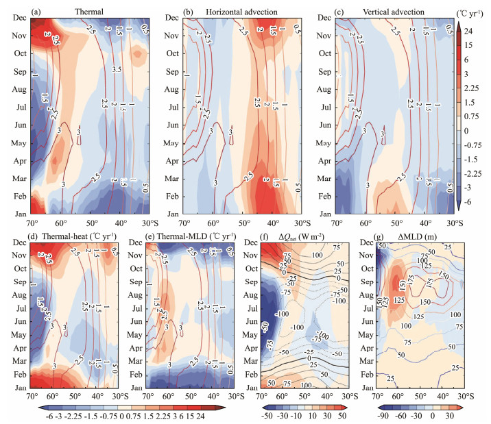
The ML heat budget for zonal-mean SO biases based on monthly mean atmospheric and oceanic variables disclose that in climatology, the thermal effect due to surface heat flux generally tends to warm the SST in both Warm-model and Cold-model ensembles (red and blue lines in Fig.8a). The effect of horizontal advection tends to cool the SO SST, primarily due to intense equatorward cold advection (red and blue lines in Fig.8b). Moreover, the vertical advection diagnosed from wind-driven Ekman pumping effect tends to decrease (increase) the SST south (north) of 50˚S (red and blue lines in Fig.8c). The residual term is relatively small, showing that the SO ML budget is primarily a balance between the surface heat flux and the ocean advection terms. The differences in these terms between the Warm-model and Cold-model ensembles (Fig.8) can represent the origins of the SO SST biases. The overall warm biases in the SO are implied to be related to an overestimated surface heating effect south of 55˚S but an underestimated cooling effect from meridional advection north of 50˚S. Indeed, there is a clear area-mean positive contribution from the thermal effect south of 50˚S and from the dynamical effect north of 50˚S (Fig.8d). Corresponding to the large seasonal variations in the SO SST biases, the excessive thermal heating effect at the high latitude primarily takes place in summertime but not wintertime (Fig.9a), while the reduced dynamical cooling effect at the low latitude are also more pronounced during summertime than wintertime for both horizontal and vertical advection (Figs.9b, 9c). Both the thermal and dynamical contribution peaks in summertime as the ML are much shallower in summertime (below 50 m) than in wintertime, which makes the ML temperature more vulnerable to heating/cooling forcing. These results determine the thermal and dynamical origin of the SO warm biases on both annual and seasonal timescales despite a relatively large residual around 30˚S and 60˚S.

Moreover, the thermal effects can be divided into two components determined by the differences in surface heat flux and MLD based on Eq. (4) (Figs.9d, 9e), which represent two different processes. At the high latitude, the improved summertime heating in the Warm-model ensemble is primarily caused by the strengthened surface heat flux (Fig.9f). In comparison, the deepened MLD (Fig.9g) under negative climatological surface net heat flux (Fig. 9f) would increase the SST from March to October by suppressing the wintertime surface cooling effect, which is clear at almost all latitudes. The results highlight the seasonal and meridional differences in the thermal processes causing the warm biases.

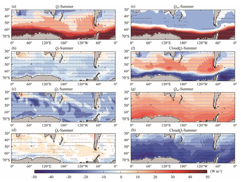
3.4 Origins of the Biases in the Thermal and Dynamical Processes

For the surface heating term diagnosed from the differences between the Warm-model and Cold-model ensembles, we show that shortwave radiation (Q_s) is dominant for the improved surface net flux and thus warm SST biases in the Warm-model ensemble than the Cold-model ensemble, which is significantly correlated with PC1 across models, especially south of 40˚S, while the other three flux terms show relatively weak or even opposite roles (Figs.10a – d). For the clear sky (noncloud) and cloud components of the surface radiation, there is a prominent positive contribution on the warm SST biases from the clear sky shortwave radiation (Q_scs) south of 60˚S (Fig.10e) and from the clear sky longwave radiation (Q_lcs) at all latitudes (Fig.10g), which aligns with the results in Fig.4 of Zhang et al. (2023). The cloud-induced shortwave radiation (CloudQ_s) primarily shows a positive contribution to the warm SST biases at 60˚ – 40˚S (Fig.10f), while the cloud-induced longwave radiation (CloudQ_l) presents a negative contribution at all latitudes (Fig.10h). It is evident that there is large cancellation between Q_lcs and CloudQ_l (Figs.10g, 10h), causing a negative contribution from longwave radiation (Q_l) (Fig.10c) and leaving the Q_s to be dominant in explaining the positive contribution from surface net heat flux south of 50˚S.

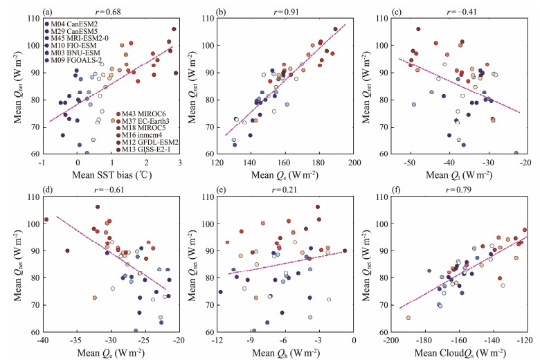
Indeed, the intermodel correlation coefficient is significantly high (0.68) between the summertime SST biases and surface net heat flux at the high latitude (Fig.10a), supporting the conclusion from the above quantitative ML budget analysis. The summertime Q_s highly correlates with Q_net (r = 0.91, Fig.11b) and SST biases (r = 0.73, not shown), indicating that at the high-latitude SO, models with high Q_s tend to induce high Q_net and therefore improve the SST. In addition, Q_l is generally opposite to Q_s and thus negatively correlates with Q_net (Fig.11c). The latent heat loss is positively correlated with Q_net (Fig.10d), primarily because the connection that increased SST would induce more latent heat loss. The sensible heat flux is negligible to the intermodel differences in Q_net (Fig.11e). Thus, only Q_s can well explain the positive intermodel correlation between SST biases and Q_net. Previous studies suggest that the overestimated Q_s is tightly related to the mispresented cloud and its effect on Q_s, which is confirmed by the high intermodel correlation of summertime cloud-induced Q_s with Q_net (r = 0.79, Fig.11f), which is consistent with Hyder et al. (2018). Furthermore, the intermodel spread in summertime surface net heat flux at 70˚ – 50˚S negatively correlated with CloudQ_l (r = −0.57) and weakly correlated with the Q_scs (r = 0.1) and Q_lcs (r = 0.38).

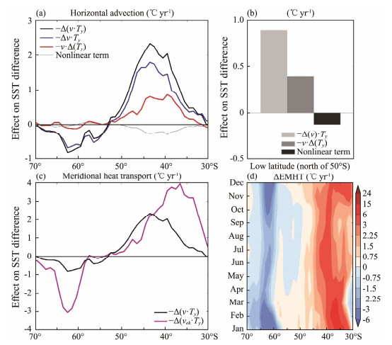
For the dynamical origin of the low-latitude SO SST biases, the horizontal advection is determined by meridional heat transport and can be decomposed into the effect of differences in meridional currents (−∆v·T_y) and temperature gradient (−v·∆T_y) based on Eq. (5) (Fig.12a). Both factors tend to result in a warmer SST north of 50˚S, but the contribution from −∆v·T_y is about two times of −v·∆T_y (Fig.12b). Also, the wind-driven Ekman heat transport (−v_ek·∆T_y) dominates the warm contribution from −v·T_y at 50˚ – 30˚S. Indeed, the warm Ekman advection persists year-round and is highly consistent with the seasonal evolution of the SST differences between the Warm-model and Cold-model ensembles (Fig.7d). The SO is dynamically controlled by the westerlies, which drives strong equatorward Ekman transport and leads to intense surface cold advection. This implies that models with large warm biases at the low latitude display weak equatorward Ekman transport and thus reduced cold advection.

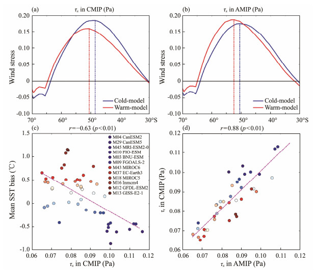
In CMIP simulations, large biases are observed in the surface zonal wind (u10m, Fig.13a). The westerlies are generally weaker at the high latitude in the Cold-model ensemble than the Warm-model one, showing substantial meridional contrast. Meanwhile, the Warm-model ensemble shows much weaker westerlies north of 55˚S than the Cold-model, consistent with their differences in meridional heat transport (Fig.12). This shows a difference in the axis of the westerlies (Fig.13a). The intermodel correlation coefficient is also significantly high (−0.63) between the surface zonal wind stress and SST biases at 50˚ – 30˚S (Fig.13c). These results suggest the crucial role of zonal wind biases in the formation of the SO SST biases at the low-latitude.

The above analyses disclose the significance of surface heat flux-related thermal origin at the high latitude and wind-related dynamical origin at the low latitude of the SO SST biases but cannot further determine whether they arise from the atmosphere or other components. We, therefore, use the outputs from AMIP to address this issue.

In AMIP simulations, the differences in surface zonal wind between the Warm-model and Cold-model ensembles are similar to that of the CMIP but with weaker differences in magnitude and the latitudinal position of the axis of the westerlies. In general, the atmosphere component of the Cold-model ensemble still simulates stronger (weaker) westerlies at the low (high) latitudes compared with that of the Warm-model ensemble despite the fact that they are all driven by observed monthly SST and sea ice. This demonstrates that the atmospheric intrinsic biases are the main origin of the westerly biases across models, and the ocean–atmospheric feedback can also amplify the wind differences. Indeed, the intermodel correlation coefficient is remarkably high (0.88) between the surface zonal wind stress from CMIP and AMIP (Fig.13d), which furtherly proves the dominant role of the atmospheric origin of the wind biases and, thus, low-latitude warm SST biases.

4 Summary and Discussion

In this work, the performance of CMIP5 and CMIP6 models in simulating the SO climatology SST has been systematically assessed by a large ensemble of models, with an emphasis on the zonal-mean results. Different from most of the previous studies, we combine models from the same community sharing highly similar SST biases and remove the effect of GMSST differences across models. The two measures are supposed to show a more accurate evaluation of the SO local SST biases in CMIP models. The findings reveal that there is an enhancement in model performances from CMIP5 to CMIP6. In particular, the MME zonal-mean local SST warm biases reduce from 0.38℃ to 0.28℃ (a decrease of around 26%), with an increase in the consistency of the models at 70˚ – 30˚S. The dominant EOF mode of the intermodel variations in the SO SST is characterized by uniform warm biases that are large at the high latitude and relatively weak at the low latitude, which explains 79.1% of the intermodel variance and shows positive principal values for most models.

The ML heat budget, based on differences between the Warm-model and Cold-model ensembles, further reveals that the pronounced summertime warm SST biases south of 50˚S primarily result from the excessive summertime heating effect from surface net heat flux, especially the surface shortwave radiation. Moreover, the cloud-induced shortwave radiation is important at 60˚ – 40˚S, while the clear sky shortwave radiation is also crucial for the formation of the SO warm SST biases south of 60˚S. The large intermodel spread in summertime surface net heat flux is tightly related to the differences in cloud-induced shortwave radiation. Meanwhile, at the low-latitude SO (north of 50˚S), the underestimated westerlies cause reduced Ekman transport and thus weakened northward cold advection, resulting in low-latitude warm SST biases. Different from seasonal varying surface heat flux biases, the low-latitude SST warm biases arising from the wind biases are apparent year-round. The critical zonal wind biases generating the SO zonal-mean SST biases can further be traced back to the AMIP simulations, i.e., atmospheric intrinsic biases. Indeed, Ceppi et al. (2012) proposed that the SH westerly jet biases may also result from biases in cloud-induced radiative forcing. These findings suggest that a more realistic simulation of the SH cloud and atmospheric circulation can largely benefit the SO SST simulation.

The focus of this work is on the characteristics and underlying processes of the SO SST biases on the zonal-mean scale. The reduced SO local SST warm biases from CMIP5 to CMIP6 and increased model consistency primarily originate from the enhancement in surface net heat flux for MME and intermodel spread (not shown); cloud and noncloud components of the surface radiation may both contribute to the differences between the two CMIPs (Zhang et al., 2023). Indeed, Figs.1 and 4 demonstrate large zonal differences in the SST biases in both CMIPs, with intense warm biases between 40˚S and 60˚S but large cold biases in the southeast of Africa, South America, Australia, and New Zealand. These zonal differences include more complicated processes and warrant further in-depth investigation. The effects of sea ice simulations in the SST biases near the Antarctic are not studied because of the complicated processes involved and calls for more in-depth investigation. Clear-sky shortwave and longwave radiation biases are crucial for the SST biases formed south of 70˚S, which is consistent with Zhang et al. (2023) and requires attention. The large-scale ocean circulation, such as the Atlantic meridional overturning circulation (AMOC), is also proposed to be connected with the SO biases (Wang et al., 2014; Luo et al., 2023) due to its regulation in the formation of North Atlantic Deep Water and Antarctic Bottom Water (Broecker, 1998; Weaver et al., 2003). However, it is worthy to mention that there is a study proposing that the relationship between the SO warm SST bias and the AMOC strengths is not statistically significant in some models (Hyder et al., 2018). Luo et al. (2023) mentioned that the simulated AMOC strength biases are not the primary cause of the SO SST warm biases but that the AMOC will serve as an adiabatic pathway to connect the North Atlantic deep ocean temperature biases with the SO SST biases. The controversial conclusions from different studies imply that the role of AMOC is highly model-dependent, perhaps due to the selection of models employed herein. Thus, it is also imperative to explore the detailed connection and processes of the AMOC simulation with the SO SST biases by combining homological models to increase model independence.

Acknowledgements

We acknowledge the World Climate Research Programme, which, through its Working Group on Coupled Modelling, coordinated and promoted CMIP5 and CMIP6. We thank the climate modeling groups for producing and making available their model output, the Earth System Grid Federation (ESGF) for archiving the data and providing access, and the multiple funding agencies that support CMIP6 and ESGF. ERSSTv5 can be downloaded through the following website: https://www1.ncdc.noaa.gov/pub/data/cmb/ersst/v5/netcdf/. CCMP Version-3.0 vector wind analyses are produced by Remote Sensing Systems. Data are available at www.remss.com. This work is supported by the National Natural Science Foundation of China (Nos. 42076208, 42141019, 41831175 and 41706026), the National Key Research and Development Program of China (No. 2017YFA0604600), the Natural Science Foundation of Jiangsu Province (No. BK20211209), and the Fundamental Research Funds for the Central Universities (Nos. B210202135 and B210201015).