1 Introduction

Changes in the climate system due to global warming are topical issues in the field of international climate research (Xu et al., 2013; Zhou et al., 2013). Observational data are an essential basis for the scientific communities in climate change research and interactions (Bromirski et al., 2005; Gemmrich et al., 2011). Long-term, high-precision, and large-scale field observations are ideal data for related research. However, on-site observations are still sparse worldwide and temporally discontinuous, particularly on coastal and open seas (Agarwal et al., 2013; Stopa and Cheung, 2014). The lack of high-quality, high-frequency, long-term, and temporally continuous global observations is one of the biggest challenges in understanding the global climate system (Guedes Soares and Scotto, 2001; Campos and Guedes Soares, 2016).

Scientists proposed using data assimilation technology in numerical weather prediction to compensate for the irregular temporal and spatial distributions of observational data and restore long-term historical climate records in the late 1980s, called 'reanalysis' of atmospheric data. Bengtsson and Shukla (1988) and Trenberth and Olson (1989) proposed that the atmospheric observational data used for climate research should first utilize the fixed dynamic system framework and assimilate the existing observational data for reanalysis. Based on this method, atmospheric data 'reanalysis' is a process that uses the data assimilation system to optimally integrate various types and sources of observational data with short-term numerical weather prediction products. Beginning in the mid-20th century, researchers from different countries and institutions initiated atmospheric reanalysis data processing programs and obtained a large amount of reanalysis data products (Hodges et al., 2003), such as the National Centers for Environmental Prediction (NCEP) reanalysis data in the United States, European Centre for Medium-Range Weather Forecasts (ECMWF) reanalysis data in Europe. The spatial and temporal resolutions, corresponding numerical models, assimilation schemes, and assimilated observations of these data products considerably differ. Most of the reanalysis data products with lower/higher horizontal resolution currently have a period of around 40/70 years (Wang et al., 2018). The emergence of reanalysis data provides the necessary support for the study of ocean and atmospheric processes (Guedes Soares and Scotto, 2001; Cardone et al., 2015). Using reanalysis data can deepen the understanding of atmospheric circulation and promote the development of atmospheric science and related research (Simmons et al., 2010; Agarwal et al., 2013; Portilla et al., 2013). However, reanalysis data use data assimilation technology to obtain forecast products after inputting observational data, which can be affected by the accuracy of the input observations. Thus, the applicability of the reanalysis data should be assessed, especially in regions where the observations are sparse, such as the western Indian Ocean (WIO) region.

East Africa has a high population and a large amount of economic development, which has continuously attracted the attention of the United Nations. The Asia-Africa-Australia monsoon system is the most active globally, affecting the Indo-Pacific region, which is the region with the highest population and frequency of economic activities. The East African monsoon is an integral part of the Asian-African-Australian monsoon system. During the summer, the cross-equatorial airflow along the coast of East Africa is a vital water vapor transport channel for the South and East Asian summer monsoon (Wang, 1999; Xu et al., 2016; Chiang et al., 2020; Li et al., 2020). Agriculture is the most important financial sector in East African countries, and the number of people engaged in agriculture is as high as 80% of the population. The export of agricultural products occupies an essential position in the foreign trade exports of various countries. Therefore, extreme weather events will cause substantial economic losses and social unrest (Lyon, 2014; Yang et al., 2014). For example, the severe drought in 2010/11 in Kenya, Somalia, and southeastern Ethiopia affected approximately 10 million people and caused more than 250000 deaths in Somalia alone (Checchi and Robinson, 2013; Kew et al., 2019). The extreme drought in 1983/1984 caused famine and one million deaths in Ethiopia and northern Sudan (Conrad, 1986; Gilkes, 1994). Compared with South Asian and Asian-Australian monsoon research, monsoon research in East Africa is less comprehensive due to sparse observations in these areas. Therefore, completely understanding and grasping the evolution characteristics of the East African monsoon system is essential for acquiring comprehensive and accurate data of the monsoon system.

The First Institute of Oceanography, the Ministry of Natural Resources, China, and the Kenya Meteorological Department jointly conducted in situ observations in East African waters and successfully deployed a Bailong buoy system (39˚41΄E, 4˚09΄S) in the WIO in September 2019, obtaining 23 days of real-time sea surface weather parameter observations. This study uses buoy observational data to compare and evaluate the current high-frequency atmospheric reanalysis products and identifies the advantages and disadvantages of each reanalysis product in reproducing the essential atmospheric variables in the WIO region.

2 Data and Methodology 2.1 Bailong Buoy Observation

Bailong buoy is a deep ocean climate observation system that was independently researched and developed on the basis of advanced international technologies brought in and assimilated by the First Institute of Oceanography, Ministry of Natural Resources, China. As a platform for open ocean climate observation, the Bailong buoy is equipped with multi-element sensors and can acquire high-frequency sampling of sea surface weather, oceanographic elements, and internal marine elements; it can then transmit the observed data to the coastal data center in Qingdao through Iridium communication (Freitag et al., 2016). Since 2010, the Bailong buoy has been successfully deployed in the East Indian Ocean and the Andaman Sea, becoming the third deep-ocean climate observation buoy system after the Tropical Atmosphere Ocean by the National Oceanic and Atmospheric Administration and the Triangle Trans-Ocean Buoy Network by the Japan Agency for Marine-Earth Science and Technology. In 2019, scientists in China and Kenya conducted joint observations and deployed a set of Bailong buoy systems in the coastal region of Kenya, which measured air temperature, humidity, rainfall, sea level pressure, surface wind, and ocean temperature and salinity. All sensors mounted in this buoy were calibrated by the National Center of Ocean Standards and Metrology. This buoy sent real-time raw data from September 1 to September 24, 2019, via satellite. To maintain the precision of the raw data, the quality of the buoy data is controlled via the following steps. First, the values of variables beyond the reasonable range (e.g., 0 – 40 m s⁻¹ for wind speed and 1005 – 1020 hPa for pressure, similar to the procedure in Wang et al. (2017) and Song et al. (2021)) are removed. Second, the missing values are linearly interpolated on the basis of the nearest samples. Third, the hourly variables are then obtained by averaging the high-resolution measurements (Song et al., 2021). The observed sea level pressure (SLP) and surface wind data are used in the current study to assess the performance of different reanalysis data in the WIO.

2.2 Reanalysis Data

This study collects international high-frequency atmospheric reanalysis data (Table 1) from different scientific organizations. The periods of reanalysis data in this study are chosen from September 1 to 23, 2019, for comparison with the observations. The variables analyzed in this study are SLP, zonal wind (Uwnd), and meridional wind (Vwnd).

ECMWF Reanalysis v5 hourly data on the single levels (ERA5 single), ECMWF Reanalysis v5 hourly data on the pressure levels (ERA5 pressure) (Hersbach et al., 2020), ECMWF Atmospheric Composition Reanalysis 4 (EAC4) (Inness et al., 2019), and Year of Polar Prediction (YOPP) are from ECMWF (Masatake et al., 2021). NCEP-NCAR Reanalysis (hereafter R-1) (Kalnay et al., 1996) and NCEP-DOE Atmospheric Model Intercomparison Project (AM-IP-II) reanalysis (hereafter R-2) are acquired from NCEP (Kanamitsu et al., 2002). The Modern-Era Reanalysis for Research and Applications, Version-2 (MERRA2) is acquired from the National Aeronautics and Space Administration (Cullather and Bosilovich, 2017; Kim et al., 2017), and the Japanese 55-year Reanalysis (JRA55) is acquired from Japan Meteorological Agency (Kobayashi et al., 2015; Harada et al., 2016).

2.3 Methodology

Statistical analysis methods are applied in the current study for the original and anomalous data, such as standard deviation, power spectrum analysis, and Taylor diagrams (Taylor, 2001). The anomalous fields are defined as the deviation of each variable from the average state during the study period (September 1 – 23). The deviation fields indicate the departure from the observations at each hour during the study period for each variable. The time interval of the buoy measurement is 1 h, and that for the different reanalysis data varies from 1 h to 12 h. The time of the observations is selected on the basis of different time intervals for each reanalysis data to perform the statistical calculation. Reanalysis data hold different spatial resolutions (Table 1). Thus, the nearest grid point to the observations is selected as the representative value for each reanalysis data (Zhang et al., 2016, Zhou et al., 2018).

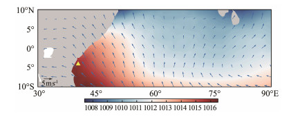
3 Results 3.1 SLP

The spatial distribution of climatological SLP in September (data from R-1) is listed in Fig.1. From the perspective of climatological conditions, SLP in the WIO is high in the west and low in the east. The maximum value appears near Tanzania and reaches 1017 hPa, and the value in the northeastern part of Sri Lanka is the minimum with a value of 1008 hPa.

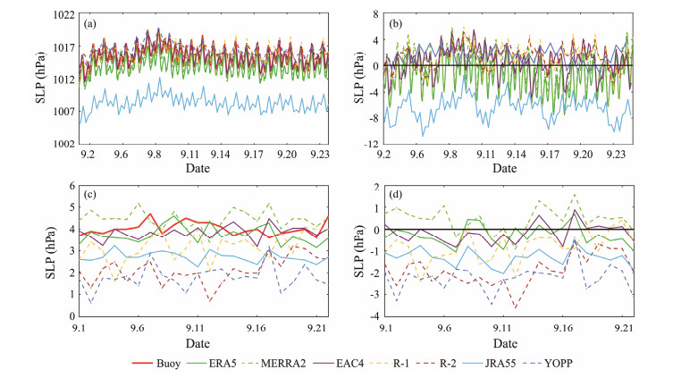
The strength of the buoy-observed SLP ranges from 1010 hPa to 1020 hPa, while most reanalysis datasets present a reasonable strength compared with the observations, except for JRA55 (Fig.2a). The JRA55 data present large deviations from the observations, and the amplitude ranges are 998 – 1005 hPa, which reveal a significant system bias for underestimating the observations. The observations show significant diurnal variation in SLP, which can be captured by all reanalysis data evaluated; however, the amplitude for each data point is quite different. The ERA5 (ERA5 single), MERRA2, EAC4, R-1, and R-2 data can effectively describe SLP evolution.

The deviation of the SLP time series is calculated to describe the detailed structure of the departure between the reanalysis data and the observation (Fig.2b). Almost all reanalysis datasets accurately describe SLP characteristics revealed by the observations, except for JRA55, and this phenomenon is also reflected in Fig.2a. The departure between MERRA2 and the observations is the minimum among all the reanalysis data. The magnitude of the diurnal change in SLP is 3.5 – 4.5 hPa in the observations during the study period (Fig.2c). Interestingly, the diurnal changes in each reanalysis data are inconsistent with the observations (Fig.2d). The variation ranges of ERA5 and EAC4 are the closest to the observations, and the ranges are 3.1 – 4.6 and 3.1 – 4.3 hPa, respectively. The descriptions of R-2 and YOPP are the most unrealistic compared with other reanalysis data for reproducing the diurnal change in SLP, which underestimates the amplitude during the entire study period. MERRA2 holds a remarkable daily variation ranging between 3.5 and 5 hPa.

The statistical features of SLP diurnal changes in each reanalysis data are further calculated on the basis of the observations (Table 2). EAC4 presents effective performance for standard deviations (STDs), and JRA55 holds the minimum standardized root mean square (RMS) error with a value of 1.2.

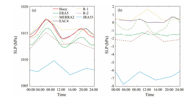
On average, a significant semidiurnal cycle is found in the observed SLP data (Fig.3a). Two maximum and minimum amplitude values occur during the whole day. The maximum SLP value occurs at approximately 06:00 and 20:00 Coordinated Universal Time (UTC), and the minimum occurs at 13:00 and 24:00 UTC, which is the significant semidiurnal tide signal (Dai and Wang, 2016). This phenomenon can be accurately captured by all datasets with double peaks of SLP amplitudes despite the two-hour delay of MERRA2 and JRA55 data for the peak time compared with the observations. This phenomenon indicates that the semidiurnal tides can be successfully reproduced in most reanalysis datasets. However, large diversity exists within the amplitude of semidiurnal changes in each reanalysis data, and the JRA55 data hold the largest diversity among the datasets, with the maximum value reaching 8 hPa (Fig.3b). EAC4 presents the best performance in averaged diurnal change.

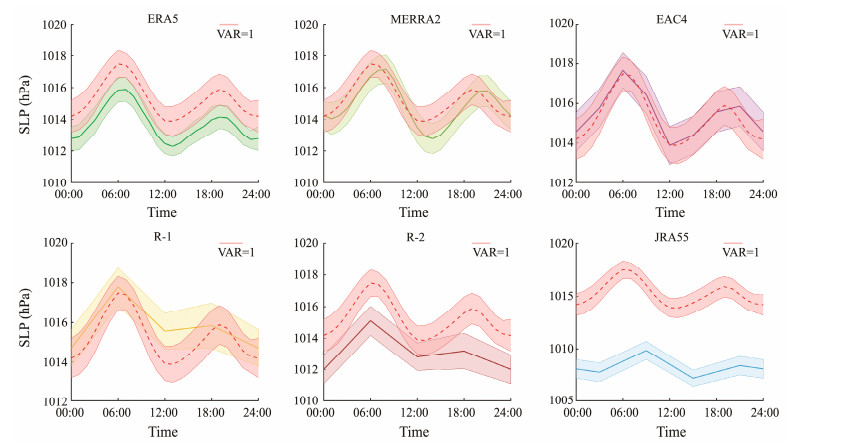
Considering the variation, the MERRA2 and EAC4 data approach the observations with similar variation amplitudes (Fig.4). The amplitudes of variation of ERA5, R-2, and JRA55 data are generally smaller than the observations. The R-1 data show a different performance with arge variance between 08:00 and 18:00 and a similar variance at other times. The ERA5 data hold the minimum variance between 06:00 and 12:00 compared with the observations, which presents a similar trend as the observations.

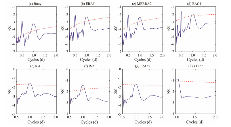
Fig.5 shows that all reanalysis datasets can describe the semidiurnal and diurnal cycles in the observations as well as the relevant variances.

The Taylor diagram can reflect the general description by jointly considering several statistical variables. The correlation coefficients indicate that MERRA2 shares the best description with the observations, with a value of 0.93. By contrast, EAC4 shows the worst correlation between observations, with a value of 0.51. The R-2 has the least STD of 0.70, and JRA55 has the largest STD with a value of 1.12. The RMS of MERRA2 is the smallest, with a weight of 0.37, and EAC4 has the largest RMS. The information revealed in Fig.6 is consistent with Fig.1.

3.2 Surface Wind

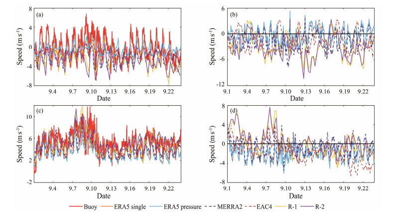
The spatial distribution of the climatological surface wind field in September is listed in Fig.1. The wind distribution in the target area of the WIO is mainly southerly. West of 48˚E, the wind flows westward to approximately 36˚E and changes into the east wind. An anticyclone field is also observed in the eastern part of the WIO (0˚ – 10˚S, 72˚ – 90˚E). The meridional wind had a larger amplitude than the zonal wind during the study period. The strength of Uwnd observations ranges from −6 to 6 m s⁻¹ while Vwnd ranges from 0 to 12 m s⁻¹, which is almost twice that of Uwnd (Figs.7a and 7b, respectively). From September 7 to 12, the buoys experienced a significant weather process with an abrupt increase in Vwnd from 6 m s⁻¹ to 12 m s⁻¹ due to a moderate strengthening of Uwnd. The variation of Vwnd indicates that meridional wind around the buoy system during the study period is primarily northward, and the direction of Uwnd changes daily with a significant breeze feature. Compared with Vwnd, the diurnal variation of Uwnd is prominent, which could be captured in all datasets (Fig.7c). Almost all reanalysis datasets significantly deviate from the observations not only in Uwnd but also in Vwnd. Regarding Uwnd, R-2 presents a significant departure from the observations, mainly from September 13 to 22 in general, and the maximum departure reaches 11 m s⁻¹ on September 13. The ranges of ERA5 single and ERA5 pressure are quite close to the observations, with a strength of −2.2 – 1.5 m s⁻¹ and −2.4 – 2.1 m s⁻¹. Except for R-2, R-1, and EAC4, the other data can describe the surface wind characteristics successfully revealed by the observations. Considering Vwnd, R-2 also shows a larger deviation compared with other data, while the maximum departure remains between September 2 and 8, with a strength reaching 8 m s⁻¹. Vwnd presents a reasonable strength from September 13 to 22 (Fig.7d). Other data present a small departure from the observations, except for EAC4, which also shows a large deviation from September 19 to 23, with the maximum value reaching −7 m s⁻¹. Another feature for Vwnd lies in the underestimated strength of all datasets during the study period, especially after September 10.

Diurnal change features are reflected in Figs.8a and 8b. Interestingly, Uwnd and Vwnd show significant increasing trends of diurnal signals between September 7 and 12, especially on September 9, wherein the maximum diurnal change occurs with the amplitudes of Uwnd and reaching 13 and 9 m s⁻¹, respectively. The abrupt increase in these diurnal changes is captured by R-1, R-2, and MERRA-2 despite the advance occurrence (2 – 3 d) of peak time of Vwnd in the reanalysis. ERA5 single, ERA5 pressure, and EAC4 fail to reproduce a similar increasing feature. All reanalysis datasets generally underestimate the diurnal changes in Uwnd and Vwnd, which is a common problem among these datasets (Figs.8c, and 8d).

The statistical variables of the diurnal change in Uwnd (Table 3) and Vwnd (Table 4) are further calculated on the basis of these observations. For Uwnd, only R-1, R-2, and MERRA2 positively correlate with the observations, while all reanalysis datasets are positive for Vwnd. The description of Vwnd is generally better than Uwnd in reanalysis data.

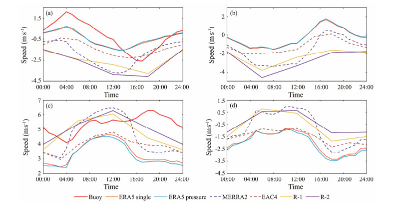
From the viewpoint of averaged conditions, all reanalysis datasets and the observations exposed an apparent diurnal cycle in the surface wind during the study period. The observed diurnal variation in Uwnd comprises a maximum and minimum value, which occurs at 04:00 and 16:00 UTC, respectively (Fig.9a). For Vwnd, the minimum and maximum values of Vwnd occur at 04:00 and 18:00 UTC, respectively (Fig.9b).

Most reanalysis datasets can accurately describe the averaged diurnal changes in the surface wind, but the peak times are quite different. For Uwnd, R-2 and R-1 present poor descriptions among all datasets since the maximum value occurs at 00:00 (4 h earlier than the observations), and the minimum value occurs at 17:00 (1 h later than the observations). MERRA2 fails to reproduce the current minimum value time, which is 12:00 (4 h earlier than the observations), and the ERA5 single and ERA5 pressure present similar conditions. All the datasets underestimate the strength of Uwnd (Fig.9c). The condition for Vwnd is different. All datasets present the maximum value at 12:00 in Vwnd, which is 6 h earlier than the observations. MER-RA2, R-2, and R-1 present stronger amplitudes than the observations at peak times, with values of 6.5, 6.3, and 6.0 m s⁻¹, respectively, and others present weaker amplitudes. The ERA5 single and ERA5 pressure present weaker amplitudes than the observations, with a value of 4 m s⁻¹. Most of the datasets underestimate the strength of Vwnd, nighttime before midnight witnessed the largest departure compared with the observations, and the maximum value reached 3.5 m s⁻¹ by ERA5 single and ERA5 pressure (Fig. 9d).

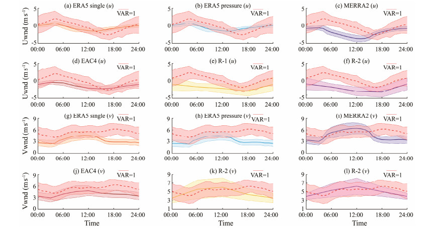
Considering variance, a large diversity occurs in each data point (Fig.10). The ERA5 pressure generally presents the weakest variation among the observations.

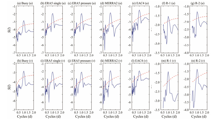
Power spectrum analysis (Fig.11) demonstrates that all reanalyses can accurately describe the diurnal cycle for the surface wind, which is consistent with Figs.9 and 10. In addition, ERA5 single, ERA5 pressure, and MERRA2 show peak periods of 0.5 and 0.25 days, which may be false.

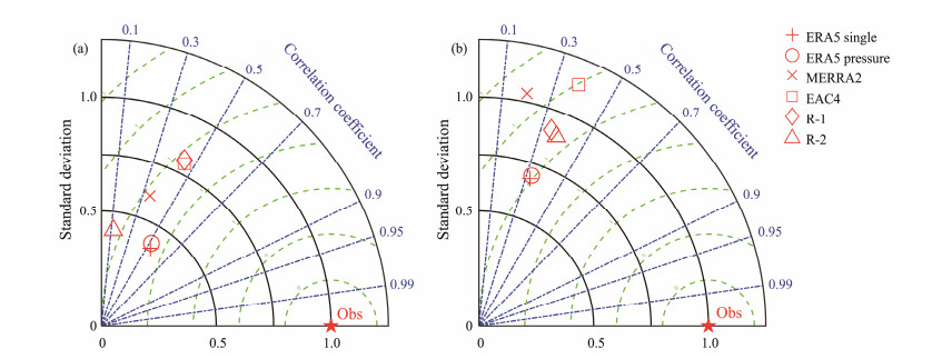
The Taylor diagram for Uwnd and Vwnd indicates that all reanalysis datasets fail to reproduce the statistical features of the observations (Fig.12). For Uwnd, R-2, ERA5 single, and ERA5 pressure present relatively poor performance in reproducing the observations. EAC4 and R-1 provide improved descriptions, and the description of MERRA2 is in the middle. For Vwnd, ERA5 single and ERA5 pressure provide poor descriptions, with EAC4 demonstrating superior performance. MERRA2 shows a poor correlation with the observations. Similar to the previous conclusion, a systematic deviation is observed in the description of the surface wind in the reanalysis data.

4 Conclusions

Based on the observational data of buoys deployed in the WIO in 2019, this research conducts a preliminary assessment of the SLP and sea surface wind from state-of-the-art high-resolution atmospheric reanalysis data. The reanalysis data in the WIO generally have a good performance when describing SLP, and the differences with the observations are slight. However, the surface wind description is poor, and meridional wind underestimates the variance and amplitude in all reanalysis datasets.

EAC4 and MERRA2 data provide superior performances from the perspective of SLP. The JRA55 data have a systematic bias of the amplitude despite its quite similar variance to the observations. The diurnal change in SLP is accurately captured by all reanalysis datasets because the double peak time of the maximum pressure value is reproduced with different amplitudes. MERRA2 generally presents a better description than SLP observations. The descriptions for the surface wind are quite different. Unlike SLP, all the reanalysis datasets underestimate the amplitudes of zonal and meridional winds, especially for meridional wind. The diurnal cycle cannot be accurately reproduced by all reanalysis datasets because the peak time of the maximum value occurs at 12:00 instead of 16:00 UTC in the observations.

Overall, from the perspective of high temporal resolution, the major atmospheric reanalysis products still have a systematic bias in describing the sea surface wind over the western tropical Indian Ocean, particularly in the meridional wind intensity description. A significant deviation is also observed in the diurnal changes. By contrast, the descriptions of SLP by reanalysis data are superior. The surface wind is important for further analyses, such as heat flux calculations, and the unrealistic performance of the surface wind may introduce errors into relevant calculations, leading to unrealistic results. This research provides a rough assessment of high-frequency wind and SLP performance in the WIO. The results can give useful information for a further study supported by the aforementioned reanalysis data in the WIO region. Reanalysis data products for research on the atmospheric environment of the WIO, especially on high-frequency surface wind changes, should be carefully treated.

Considering that the buoy observations in this study obtained data for only 23 days, the obtained results can only quantitatively reveal the performance of each reanalysis data product in September 2019 instead of the entire period of different reanalysis data. The inapplicability of these results in other seasons or years is possible. Therefore, the results of this study have certain limitations considering the aforementioned circumstance. In the future, additional field observations should be used for further analysis and should provide additional information on the applicability of high-frequency reanalysis data in the western tropical Indian Ocean.

Acknowledgements

This work was supported by the Global Change and Air-Sea Interaction Program (No. GASI-04-QYQH-03), the Taishan Scholars Program of Shandong Province (No. tsqn201909165), the National Natural Science Foundation of China (No. 41876028), the Global Change and Air-Sea Interaction Program (No. GASI-01-WIND-STwin), the Shan-dong Science and Technology Foundation (No. 2013GRC31504), and the Marine S & T Fund of Shandong Province for Pilot National Laboratory for Marine Science and Technology (Qingdao) (No. 2022QNLM010103-3).