1 Introduction

Jacket-type platform, a common structural system used in shallow water, plays a crucial role in offshore oil and gas development. In recent years, this type of structure has been widely employed as a supporting structure for offshore wind turbines (Wei et al., 2016). Alessi et al. (2019) investigated the possibility of converting actual structures for gas extraction into offshore platforms for wind turbine towers. Compared with land-based steel jacket structures, water-based jacket structures face more complex environmental conditions, such as wind, waves, currents, ice, and earthquakes. Vahdati et al. (2020) conducted an experimental study to investigate combined solutions to reduce scouring around complex foundations. Moreover, due to the strong hydrodynamic interaction effects faced by water-based jacket platforms during their service lifetime, dynamic response analysis for such platforms is essential in the design stage (Tian et al., 2019). Mourão et al. (2020) performed a combined fatigue damage evaluation using local damage parameters for an offshore jacket-type structure. Meng et al. (2020) conducted reliability-based optimization for offshore structures using saddlepoint approximation. To perform an accurate analysis of offshore structures, we have to define the anticipated extreme loads at design time using reasonable metocean extreme-condition design criteria. Thus, precise estimates of long-term extreme metocean parameters based on measured or hindcast data are important in the design and subsequent operation of offshore structures (Bruserud et al., 2018).

Normally, the safety of an offshore jacket platform must be ensured throughout the operation period. Wind or wave parameters with a 50- or 100-year return period, based on the statistical analysis of individual environmental variables, are generally adopted as extreme conditions for jacket platforms in traditional design criteria (DNV-RPC205, 2012). However, the dependency between various ocean parameters, such as wind and wave, wave height and wave period, should be considered to estimate accurate structural response and provide a realistic reliability prediction. For this purpose, joint probability distributions of various ocean parameters have been the focus of attention in recent studies. Although excellent fitting results have been produced using different joint distribution models proposed on the basis of different theories in the literature, no unifying benchmark exists for establishing joint models of metocean parameters (Jonathan and Ewans, 2013). Thus, the hybrid lognormal-Weibull conditional distribution model for significant wave height and wave period, proposed by Haver (1985), is widely accepted. Many researchers have investigated and discussed the joint distribution of other metocean parameters, such as wind speed, wave height, and current velocity, on the basis of conditional models (Belberova and Myrhaug, 1996; Bitner-Gregersen, 2005, 2015). Copula functions, which can be conveniently used to construct multivariate distributions of environmental variables using marginal distributions, are applied increasingly in sea state assessment (De Michele et al., 2007). Tao et al. (2013) estimated design parameters of wave height and wind speed using bivariate copulas. Vanem (2016) presented joint statistical models for significant wave height and wave period based on copula techniques, with results demonstrating large variability. This condition implies significant uncertainties in the estimated joint models, even for the same data, due to different modeling choices. Jonathan and Ewan (2013) provided a comprehensive review of multivariate modeling of extreme ocean parameters for marine design, highlighting that tail estimation for extreme value analysis is inherently difficult in empirical modeling.

Due to lack of knowledge necessary for constructing multi-load estimates, a simple combination of single extreme parameters obtained from the marginal distribution is widely used in the design of marine structures. The American Petroleum Institute code (API, 1995) proposed three approaches to the construction of criteria to define design loads for a fixed offshore platform: 1) combinations of 100-year wind speed, 100-year current velocity, and 100-year wave height; 2) 100-year wave height with concomitant wind speed and current velocity; 3) any reasonable combination of wind speed, wave height, and current velocity, which will result in a 100-year structural response, such as base shear force and overturning moment. These design loads are commonly treated as conservative to guarantee the safety of marine structures for their intended service lives. A widely used environmental contour approach is presented to investigate the logical multi-loads acting on the offshore structures. Notably, environmental contours determined using different joint models are expected to produce different design parameters. Haver and Winterstein (2009) constructed environmental contour lines for significant wave height and peak period using conditional models. Silva-González et al. (2013) developed 3D environmental contours using Nataf distribution for significant wave height, peak period, and wind speed. Huseby et al. (2013) presented an approach to environmental contours for significant wave height and peak period based on direct Monte Carlo simulations. Montes-Iturrizaga and Heredia-Zavoni (2015) applied copulas to develop environmental contours for bivariate metocean variables.

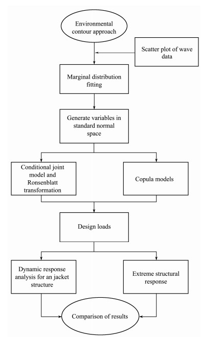
In this study, we propose a method to determine design loads for a jacket-type offshore platform based on an environmental contour technique. The flowchart in Fig.1 shows how this procedure is applied to estimate design loads for jacket structures. A brief description of environmental contour theory leads to an analytical derivation of the construction of an environmental contour model expressed on the basis of conditional joint distribution and copula models. In the next step, additional copula classes are adopted and environmental contours are constructed using a variety of models. The proposed procedure is then applied, and the results examined, using measured wave data from the United States coast. The statistical parameters of joint distribution are estimated, and goodness-of-fit tests are conducted to enable the selection of optimal copula models. Finally, extreme environmental loads are computed and the results discussed along with a jacket-platform dynamic response analysis.

2 Environmental Contour Approach

An iterative approach such as first-order reliability method (FORM) for structural failure probability analysis is computationally expensive. Winterstein et al. (1993) proposed an environmental contour approach to determine environmental parameters for extreme structural response analysis based on Inverse FORM. In this section, a brief introduction is presented on how the basic environmental contours can be constructed. Copula theory is adopted and analytical formulations of environmental contours based on various copulas are derived in later study. In the regular approach to structural reliability analysis, uncertainties in environmental loads and structural extreme responses must be considered. The key advantage of this approach is that those uncertainties can be approximately decoupled. Various environmental parameters are employed to describe the loads acting on offshore structures at a site, such as wave height and period, wind speed, current velocity, and directions of these variables. In this case, we assume a vector of two random environmental variables, X = (H_s, T_z), corresponding to an exceeding probability P_f associated with a reliability index β:

$ {P}_{f}=\frac{{T}_{s}}{365\times 24\times {T}_{r}}, $

(1)

$ \beta ={\Phi }^{-1}(1-{P}_{f}), $

(2)

where T_s represents the data sampling interval, and T_r denotes the target return period that is defined in design criteria. In structural reliability design, the failure probability P_f corresponds to a known structural response capacity y_c, where P_f = P (y > y_c), and the reliability index β denotes the shortest distance from original point to failure domain in standard normal space.

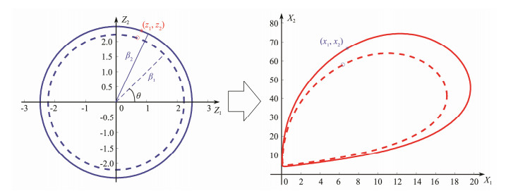
The reliability index β, in IFORM, denotes a constant radius in a standard normal space. Then, the environmental contour line in the standard normal space with a radius β can be determined, and the bivariate independent random variables, z= (z₁, z₂), which vary with angle θ, can be given as

$ {z}_{1}^{2}+{z}_{2}^{2}={\beta }^{2}\Rightarrow \left\{ \begin{array}{l}{z}_{1}=\beta \mathrm{cos}\theta \\ {z}_{2}=\beta \mathrm{sin}\theta \end{array} \right..$

(3)

Here, the vector of random variables z in the standard normal space can be transformed from original variables x = (x₁, x₂) in the original space using Rosenblatt transformation (Rosenblatt, 1952) as follows:

$ \left\{ \begin{array}{l}{z}_{1}={\Phi }^{-1}({F}_{{X}_{1}}({x}_{1}))\\ {z}_{2}={\Phi }^{-1}({F}_{{X}_{2}|{X}_{1}}({x}_{2}|{x}_{1}))\end{array} \right.\Rightarrow \left\{ \begin{array}{l}{x}_{1}={F}_{{}_{{X}_{1}}}^{-1}(\Phi ({z}_{1}))\\ {x}_{2}={F}_{{}_{{X}_{2}|{X}_{1}}}^{-1}(\Phi ({z}_{2})|{x}_{1})\end{array} \right., $

(4)

where Φ(·) is the cumulative distribution function (CDF) of the standard normal distribution, $ {F}_{{X}_{1}}({x}_{1})$ is the CDF of original variable x₁, and $ {F}_{{X}_{2}|{X}_{1}}({x}_{2}|{x}_{1})$ is the CDF of the conditional distribution of x₂ given X₁ = x₁. Fig.2 illustrates random variables in standard normal space (z) and corresponding environmental contours in physical space (x). In this example, based on return periods of 50 and 100 years, the random variable x₁ is assumed to follow a Weibull distribution in which the scale and shape parameters are 4.64 and 1.12, respectively, and variable x₂|x₁ is assumed to follow lognormal distribution in which the mean value and standard deviation are 2.87 and 0.58, respectively, and the correlation coefficient is ρ₁₂ = 0.66. The procedure and method for distribution fitting are introduced in Section 4 along with measured wave data from moored buoys.

3 Definition of Environmental Contours Using Copulas 3.1 Copula Theory

A multivariate joint distribution can be obtained from several univariate marginal distributions using copula functions. The advantage of this approach is that it can flexibly construct a joint distribution of environmental variables with arbitrary marginal distribution, and the marginal distribution and correlation structure can be considered separately, an approach that is suitable for both positive and negative correlation. A brief introduction to basic copula theory follows. We assume that $ {F}_{{X}_{i}}({x}_{i})$ are marginal distributions of the vector of random variables x = (x₁, x₂, …, x_n); if the marginal distributions are continuous, then the joint distribution function $ {H}_{{X}_{1}, \cdot \cdot \cdot, {X}_{n}}$ (x₁, x₂, …, x_n) of x can be expressed following Sklar's theorem as follows (Sklar, 1959; Zhai et al., 2017):

${H}_{{X}_{1}, \cdot \cdot \cdot, {X}_{n}}({x}_{1}, {x}_{2}, \cdot \cdot \cdot, {x}_{n})=C({F}_{{X}_{1}}({x}_{1}), {F}_{{X}_{2}}({x}_{2}), \cdot \cdot \cdot, {F}_{{X}_{n}}({x}_{n}))\\ \ \ \ \ \ \ \ \ \ \ \ \ \ \ \ \ \ \ \ \ \ \ \ \ \ \ \ \ \ \ \ \ \ \ \ \ \ \ \ \ =C({u}_{1}, {u}_{2}, \cdot \cdot \cdot, {u}_{n}), $

(5)

where C(·) represents a copula function that is monotonic and non-decreasing; it can be defined by joint distribution and inverse CDF of marginal distribution as follows:

$ C({u}_{1}, {u}_{2}, \cdot \cdot \cdot, {u}_{n})={H}_{{X}_{1}, \cdot \cdot \cdot, {X}_{n}}({F}_{{}_{{X}_{1}}}^{-1}({u}_{1}), {F}_{{}_{{X}_{2}}}^{-1}({u}_{2}), \cdot \cdot \cdot, {F}_{{}_{{X}_{n}}}^{-1}({u}_{n})), $

(6)

where $ {u}_{i}={F}_{{X}_{i}}({x}_{i})$ denotes the CDF of random environmental variables x. The density function can be obtained by its partial derivative of u:

$ c({u}_{1}, {u}_{2}, \cdot \cdot \cdot, {u}_{n})=\frac{{\partial }^{n}C({u}_{1}, {u}_{2}, \cdot \cdot \cdot, {u}_{n})}{\partial {u}_{1}\cdot \cdot \cdot \partial {u}_{n}}.$

(7)

The conditional distribution of x_i used in Eq. (4) can be expressed as

${H}_{{X}_{i}|{X}_{1}, \cdot \cdot \cdot, {X}_{i-1}}({x}_{i}|{x}_{1}, \cdot \cdot \cdot, {x}_{i-1})=C({u}_{i}|{u}_{1}, \cdot \cdot \cdot, {u}_{i-1})\\ \ \ \ \ \ \ \ \ \ =\frac{{\partial }^{i-1}C({u}_{1}, \cdot \cdot \cdot, {u}_{i}, 1, \cdot \cdot \cdot, 1)/\partial {u}_{1}\cdot \cdot \cdot \partial {u}_{i-1}}{{\partial }^{i-1}C({u}_{1}, \cdot \cdot \cdot, {u}_{i-1}, 1, \cdot \cdot \cdot, 1)/\partial {u}_{1}\cdot \cdot \cdot \partial {u}_{i-1}}.$

(8)

The parameter θ of copula functions represents the correlation between random variables x; once the parameter is obtained, the copula function C(·) is determined. The maximum likelihood method is a common parameter estimation method. For bivariate variables, the relationship between Kendall's τ and θ is simple; thus, the parameter can be defined as

$ {\tau }_{i}=g({\theta }_{i}), $

(9)

where Kendall's τ can be calculated using measured or hindcast datasets. Kendall's τ is used to describe the degree of dependency of random variables, and this parameter is utilized to evaluate the dependence among wave data. We let {(x₁, y₁), (x₂, y₂), …, (x_n, y_n)} represent the bivariate data of random variables (X, Y); if x_i < x_j and y_i < y_j, or x_i > x_j and y_i > y_j, then the data are concordant; otherwise, they are discordant. The Kendall's τ can be defined as (Li et al., 2013; Zhai et al., 2017):

$ \tau =\frac{a-b}{n(n-1)/2}, $

(10)

where a and b denote the number of concordant and discordant pairs, respectively, and n is the total number of data pairs.

3.2 Contour Plots Using Copulas

Once the target return period T_r is given, the radius β of the hypersphere can be defined using Eq. (1) in Eq. (2). Then, the environmental contours can be determined by mapping the standard normal space z to the original space of environmental variables x using Rosenblatt transformation. Combining Eqs. (8) and (4), the CDF of marginal distribution of environmental variables x in physical space can be expressed by inverse transformation of copula function C⁻¹(·) as follows:

$ \left\{ \begin{array}{l}{u}_{1}=\Phi ({z}_{1}) \\ {u}_{2}={C}_{{X}_{2}|{X}_{1}}^{-1}(\Phi ({z}_{2})|{u}_{1}) \\ \cdot \cdot \cdot \\ {u}_{n}={C}_{{X}_{n}|{X}_{1}, \cdot \cdot \cdot, {X}_{n-1}}^{-1}(\Phi ({z}_{n})|{u}_{1}, {u}_{2}, \cdot \cdot \cdot, {u}_{n-1}) \end{array} \right..$

(11)

Once u_i is defined, the environmental variables x_i in original space can be determined by inverse transformation of marginal CDF, $ {x}_{i}={F}_{{X}_{i}}^{-1}({u}_{i})$, and the corresponding environmental contour can be obtained. A bivariate variable example is adopted to illustrate the procedure. We assume that C(u, v) is the bivariate copula function. Then,

$ u=\Phi ({z}_{1}), $

(12)

$ v={C}_{v|u}^{-1}(\Phi ({z}_{2})|u)={C}_{v|u}^{-1}(\Phi ({z}_{2})|\Phi ({z}_{1})).$

(13)

For bivariate variables, the most important step is to solve the partial derivatives of copula functions, C(v|u) = ∂C(u, v)/∂u. A variety of copula functions can be applied to the establishment of bivariate joint distribution of environmental variables, such as Archimedean and elliptic copula functions. In the next section, we derive the specific expressions for v for some classes of bivariate copula functions.

3.2.1 Gaussian copula

The Gaussian copula function is given as

$ C(u, v)=\Phi ({\varphi }^{-1}(u), {\varphi }^{-1}(v)), $

(14)

where ϕ⁻¹(·) is the inverse function of standard normal distribution. The marginal distribution of random variables should follow a standard normal distribution, while the actual situation may not. Nataf transformation is a mathematical model that completes the transformation process from the original variable space to the independent standard normal space:

$ \Phi ({y}_{i})={F}_{i}({x}_{i})\Rightarrow {y}_{i}={\Phi }^{-1}({F}_{i}({x}_{i})), $

(15)

where x is the vector of target variables, x = (x₁, x₂, …, x_n)^T; F_i(x_i) represents the CDF of random environmental variables; y is the standard normal random vector corresponding to x, y = (y₁, y₂, …, y_n)^T; Φ(·) and Φ⁻¹(·) are CDF and inverse CDF of the standard normal random vectors, respectively.

Silva-Gonzláez et al. (2013) presented an environmental contour approach using the Nataf distribution model. The expression of v is given as

$ v=\Phi (\sqrt{1-{\rho }^{2}}{z}_{2}+\rho {z}_{1}), $

(16)

where ρ is the Pearson coefficient of variables in transformed standard normal space. Kendall's τ can be calculated from

$ \tau =2\mathrm{arcsin}(\rho)/\text{π}.$

(17)

3.2.2 Frank copula

The Frank copula refers to a certain family of Archimedean copula. It is defined as

$ C(u, v)=-\frac{1}{\theta }\mathrm{ln}\left[1+\frac{({\text{e}}^{-\theta u}-1)({\text{e}}^{-\theta v}-1)}{{\text{e}}^{-\theta }-1}\right], \text{ }\theta \in R.$

(18)

The relationship between parameter θ and Kendall's τ is determined as

$ \tau =1-4/\theta +4/{\theta }^{2}{\displaystyle {\int }_{0}^{\theta }s/({\text{e}}^{s}-1)\text{d}s}.$

(19)

The conditional bivariate Frank copula function can be given as

$ C(v|u)=\frac{({\text{e}}^{-\theta u}-1)({\text{e}}^{-\theta v}-1)+({\text{e}}^{-\theta v}-1)}{({\text{e}}^{-\theta u}-1)({\text{e}}^{-\theta v}-1)+({\text{e}}^{-\theta }-1)}.$

(20)

Using Eq. (16) in Eq. (13), we can present the specific expression for v as

$ v=-\frac{1}{\theta }\mathrm{ln}[1+\text{Φ}({z}_{2})\frac{({\text{e}}^{-\theta }-1)}{1+({\text{e}}^{-\theta u}-1)(1-\Phi ({z}_{2}))}].$

(21)

3.2.3 Clayton copula

The Clayton copula can be expressed by the following equation:

$ C(u, v)={({u}^{-\theta }+{v}^{-\theta }-1)}^{-1/\theta }, \text{ }\theta \in (0, \infty).$

(22)

The τ = g(θ) is defined as

$ \tau =\frac{\theta }{\theta +2}, $

(23)

and

$ C(v|u)={({u}^{-\theta }+{v}^{-\theta }-1)}^{-1/\theta -1}{u}^{-\theta -1}.$

(24)

The specific expression for v is obtained by

$ v={\left[{(\Phi ({z}_{2})/{u}^{-\theta -1})}^{-\theta /(1+\theta)}+1-{u}^{-\theta }\right]}^{-1/\theta }.$

(25)

3.2.4 Ali-Mikhail-Haq copulas

The Ali-Mikhail-Haq (AMH) copula is expressed as follows:

$ C(u, v)=\frac{uv}{1-\theta (1-u)(1-v)}, \text{ }-1\le \theta \le 1.$

(26)

Then,

$ C(v|u)=\frac{\theta uv(v-1)}{{[\theta (u-1)(v-1)-1]}^{2}}-\frac{v}{\theta (u-1)(v-1)-1}, $

(27)

$ \tau =1-\frac{2\left[\theta +{(1-\theta)}^{2}\mathrm{ln}(1-\theta)\right]}{3{\theta }^{2}}.$

(28)

Note from Eq. (28) that because −1 ≤ θ ≤ 1, the approximate range of τ is −0.1817 ≤ τ ≤ 1/3. Thus, the application of the AMH copula is limited.

The v can be determined by

$ v=\frac{-b-\sqrt{{b}^{2}-4ac}}{2a}, $

(29)

where

$ \left\{ \begin{array}{l}a={(\theta u-\theta)}^{2}\Phi ({z}_{2})-\theta \\ b=-2{\theta }^{2}{u}^{2}+4{\theta }^{2}u-2{\theta }^{2}-2\theta u+2\theta \\ c={\theta }^{2}{u}^{2}-2{\theta }^{2}u+{\theta }^{2}+2\theta u-2\theta +1 \end{array} \right..$

(30)

3.2.5 Farlie-Gumbel-Morgenstern copula

The Farlie-Gumbel-Morgenstern (FGM) copula is expressed as

$ C(u, v)=uv+\theta uv(1-u)(1-v), \text{ }-1\le \theta \le 1, $

(31)

and

$ \tau =\frac{2}{9}\theta, $

(32)

$ C(v|u)=v+\theta v(1-v)(1-2u).$

(33)

As with the AMH copula, the value range of τ is [−2/9, 2/9]. Thus, once the bivariate variables have a higher degree of dependence, this class of copula becomes unsuitable. The expression of v can be obtained using Eq. (33) in Eq. (13) as follows:

$ v=\frac{1+\theta (1-2u)-\sqrt{{\left[1+\theta (1-2u)\right]}^{2}-4\theta (1-2u)\Phi ({z}_{2})}}{2\theta (1-2u)}.$

(34)

3.2.6 Independent copula

Once the random variables are independent, τ = 0, the independent copula is adopted in the following:

$ C(u, v)=uv.$

(35)

Then,

$ C(v|u)=v, $

(36)

$ v=\Phi ({z}_{2}).$

(37)

3.2.7 Empirical copula

The empirical copula is widely used for testing goodness-of-fit. The bivariate empirical copula is defined as

$ {C}_{n}(\frac{i}{n}, \frac{j}{n})=\frac{a}{n}, $

(38)

where a denotes the number of data that satisfy x ≤ x_i and y ≤ y_i in sample (x, y), and x_i and y_i, 1 ≤ i, j ≤ n, are order statistics.

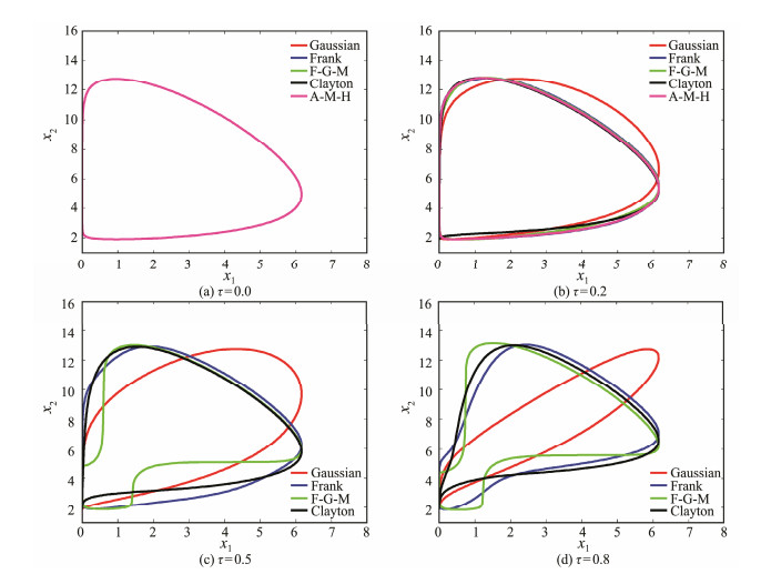
3.3 Contour Plots for Different Degrees of Dependency

In this section, we investigate the environmental contours using various copula models with different values of Kendall's τ. Based on bivariate variables (X, Y), the marginal distribution of X follows a Weibull distribution with scale and shape parameters of 1.2 and 1.6, respectively. Random variable Y is modeled as lognormal distribution in which the mean value is 1.6 and the standard deviation is 0.2. Environmental contours for T_r = 100 years (T_s = 1 h) with values of Kendall's τ equal to 0.0, 0.2, 0.5, and 0.8 are obtained using $ x={F}_{X}^{-1}(u)$ and $ y={F}_{Y}^{-1}(v)$. Fig.3 shows the environmental contours for copulas including Gaussian, Frank, FGM, Clayton, and AMH with different values of τ. The results of this example indicate the obvious differences of curves with the increase of degree of dependence. When τ = 0.0, all the copulas match the independent copula. The larger the values of Kendall's τ, the greater is the difference in the shapes of contours obtained from different classes of copula. For variables with high degrees of dependence, only the Gaussian, Frank, and Clayton copulas can describe the contour plots. Due to being limited to the size of the τ value, FGM and AMH copulas are only suitable to model environmental contours for variables with low degrees of dependence. There-fore, after constructing a joint distribution model using copula functions, we have to test the goodness-of-fit to determine whether the distribution can describe the original data identically.

3.4 Goodness-of-Fit Tests

To select the optimal joint distribution model, the most widely used method is to test the fit between the theoretical and measured values. The root mean square error (RMSE) and Akaike's information criterion are adopted to determine the most suitable copula functions.

$ RMSE=\sqrt{MSE}=\sqrt{\frac{1}{n}{\displaystyle \sum _{i=1}^{n}{\left[{p}_{c}(i)-{p}_{0}(i)\right]}^{2}}}, $

(39)

$ AIC=n\mathrm{ln}(MSE)+2k, $

(40)

where n is the sample size, p_c is the measured probability value that can be obtained from Eq. (38), p₀ is the probability value calculated from copula functions, and k is the number of parameters.

4 Case Study

A detailed description of design loads for offshore structures based on joint probability distribution of significant wave height (H_s) and zero-up-crossing period (T_s) is provided in this section. Three measured datasets (A, B, and C) gathered from the coast of the US are used. Table 1 lists the basic metadata for these datasets. All the data were sourced from moored buoys set up by the US National Oceanic and Atmospheric Administration. For data sources and a detailed introduction, refer to Haselsteiner et al. (2019). This exercise draws on 10 years worth of hourly wave data and investigates the environmental design parameters using different design criteria.

4.1 Marginal Distribution of Wave Data

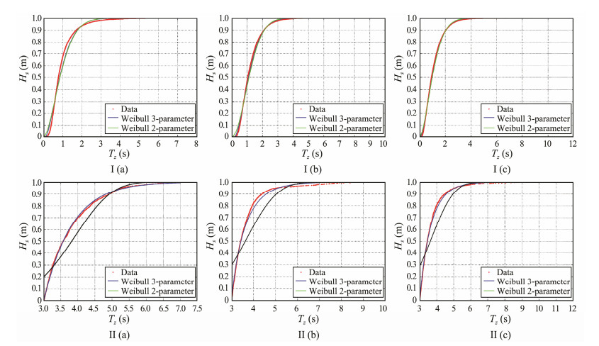
Fig.4 shows the scatter plot corresponding to datasets A, B, and C. Several distribution models were considered to fit the marginal distribution of H_s and T_z, including two- and three-parameter Weibull distribution, and lognormal distribution (Bruserud et al., 2018). The maximum likelihood method is used to estimate all the distribution parameters. Figs. 5(Ⅰ) and 6 show the empirical and fitted distributions of all H_s and T_z data. The Kolmogorov-Smirnov test indicates that all three distributions are acceptable for wave parameters. Fig.5(Ⅱ) depicts the empirical and fitted two- and three-parameter Weibull distributions for all data points of H_s exceeding a threshold of 3 m, to show the accuracy of extreme environmental parameter estimation. A total of 1455, 1836, and 1724 data points that exceed 3 m were identified at three different locations. The results indicated three-parameter Weibull distribution to be the most suitable to describe the data.

To estimate 100-year extreme parameters, one can calculate a sea state with 100-year H_s level, and the associated values of other environmental variables. The target H_s value with return period H_s can be estimated as follows using IFORM theory (Winterstein et al., 1993):

$ \beta ={\Phi }^{-1}(1-\frac{1}{365\times 24\times 100})\text{=}4.73, $

(41)

$ {H}_{s}={F}_{{H}_{s}}^{-1}(\Phi (\beta)).$

(42)

The 100-year H_s values obtained from the two- and three-parameter Weibull distributions over three locations were (5.61 m, 5.25 m), (6.04 m, 5.45 m), and (6.31 m, 6.04 m), respectively. This condition indicates that the three-parameter Weibull distribution provides a more conservative estimation than the two-parameter Weibull distribution. Based on the above factors, the three-parameter Weibull distribution and the lognormal distribution were selected to model the marginal distribution of H_s and T_z, respectively. Thus,

$ {f}_{{H}_{s}}(h)=\frac{\eta }{\alpha }{\left(\frac{h-\gamma }{\alpha }\right)}^{\eta -1}\mathrm{exp}\left(-{\left(\frac{h-\gamma }{\alpha }\right)}^{\eta }\right), $

(43)

$ {f}_{{T}_{p}}(t)=\frac{1}{\sqrt{2\text{π}}{\sigma }_{1}t}\mathrm{exp}\left(-\frac{1}{2}{\left(\frac{\mathrm{ln}\ t-{\mu }_{1}}{{\sigma }_{1}}\right)}^{2}\right), $

(44)

where h and t are target variables representing significant wave height and zero-up-crossing period, respectively; α, η, and γ are scale parameter, shape parameter, and location parameter; and μ₁ and σ₁ are mean value and standard deviation of ln(T_z), respectively. The distribution parameters estimated using the maximum likelihood method are listed in Table 2.

4.2 Conditional Distribution of T_z Given H_s

Haver and Nyhus (1986) proposed a conditional lognormal distribution to model the T_z data with parameters that correlate to H_s. Their distribution model considers the dependency between two wave parameters and is applied widely. A lognormal distribution is adopted to fit the T_z data for given classes of H_s, which still follow three-parameter Weibull distribution as in Eq. (43). Thus, the joint distribution of the wave data can be expressed as follows:

$ {f}_{{T}_{p}|{H}_{s}}(t|h)=\frac{1}{\sqrt{2\text{π}}\sigma t}\mathrm{exp}\left\{-\frac{{\left(\mathrm{ln}\ t-\mu \right)}^{2}}{2{\sigma }^{2}}\right\}, $

(45)

$ {f}_{{H}_{s}, {T}_{p}}(h, t)={f}_{{H}_{s}}(h)\cdot {f}_{{T}_{p}|{H}_{s}}(t|h).$

(46)

The parameters μ and σ are functions of h, where

$ \mu \text{=}E\left[\mathrm{ln}\ {T}_{z}\right]={f}_{1}(h), $

(47)

$ {\sigma }^{2}\text{=}Var\left[\mathrm{ln}\ {T}_{z}\right]={f}_{2}(h).$

(48)

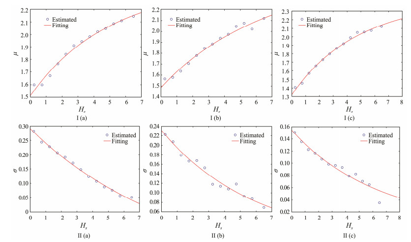
To estimate the functions of f₁(h) and f₂(h), a number of steps must be followed. First, the T_z data is divided into different classes corresponding to H_s at an interval of 0.5 m. Then, the mean value, μ_i, and standard deviation, σ_i, of lnt given a significant wave height, h_i, are estimated using the maximum likelihood method. The fitting curves of lognormal distribution parameters for given classes of H_s are then determined using least-squares regression as shown in Fig.7. The number of T_z corresponding to H_s > 7 m is extremely small, so it is ignored to avoid large divorce points affecting the fitting precision.

The estimated lognormal distribution parameters, μ and σ, are expressed by exponential functions of H_s as follows:

$ \mu ={f}_{1}(h)={a}_{1}\mathrm{exp}(-{b}_{1}h)+{c}_{1}, $

(49)

$ {\sigma }^{2}\text{= }{f}_{2}(h)={a}_{2}\mathrm{exp}(-{b}_{2}h)+{c}_{2}.$

(50)

The fitting coefficients are listed in Table 3.

In this section, the related environmental variables in physical space refer to the significant wave height H_s and zero-up-crossing period T_z, corresponding to the standard Gaussian variables z₁ and z₂, which can be defined using the following Rosenblatt transformation:

$ \left\{ \begin{array}{l}\Phi ({z}_{1})={F}_{{H}_{s}}({h}_{s})\\ \Phi ({z}_{2})={F}_{{T}_{z}|{H}_{s}}({t}_{z}|{h}_{s})\end{array} \right.\Rightarrow \left\{ \begin{array}{l}{h}_{s}={F}_{{H}_{s}}^{-1}(\Phi ({z}_{1}))\\ {t}_{z}={F}_{{T}_{z}|{H}_{s}}^{-1}(\Phi ({z}_{2}))\end{array} \right..$

(51)

Fig.8 shows the 100-year return period wave contours based on a Rosenblatt transformation using a hybrid lognormal–Weibull conditional distribution model.

4.3 Environmental Contours Using Copulas

The Kendall's τ of each of the three locations is calculated using Eq. (10) to evaluate the degree of dependence of wave data. The Kendall's τ values of (H_s, T_z) are 0.16, 0.25, and 0.47, for datasets A, B, and C, respectively, indicating that variables of all the cases are positively associated and dataset C has a relatively strong degree of dependency. Therefore, FGM and AMH copulas are not suitable for this case. The parameter θ of copula functions is calculated using τ = g(θ). Fig.8 shows the contour plots of (H_s, T_z) with a 100-year return period considering Gaussian, Frank, FGM, Clayton, AMH, independent copulas, and conditional distributions. The contour plots differ more greatly for dataset C than for datasets A and B.

For offshore structure design, a common requirement is that only a limited set of sea states can be design loads to ensure structural safety. To estimate jacket platform extreme responses in this study, we regard the design loads as environmental conditions with a 100-year return period level, H_s¹⁰⁰, which can be determined using Eqs. (41) and (42), with the representative wave period adopted as T_z = [T_zi|H_s = H_s¹⁰⁰] on the environmental contour. The design wave parameters defined for different design criteria are listed in Table 4.

The environmental contours and design wave parameters differ from classes of distribution models. The RMSE and AIC are used to select the appropriate joint probability distribution model. The test results are listed in Table 5. For all three locations, the lowest RMSE values indicate that the Frank copula function is the best model to represent joint distribution describing the wave data. AIC values support the same conclusion. Therefore, the Frank copula was selected as the distribution to represent the data for (H_s, T_p).

5 Response Analysis for Jacket Platform

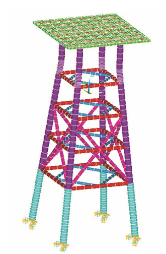
In this section, an example jacket platform is adopted to assess the dynamic response using different environmental design parameters. The jacket structure plan specifies dimensions of 12.28 m × 12.28 m at mud line elevation and a slope of 1:10. The jacket-platform work elevation is 12.0 m, the mud line elevation is −15.8 m, and static water level elevation is 0 m. A general configuration modeled jacket structure created using ANSYS software is shown in Fig.9, and the sizes of the main components are listed in Table 6.

5.1 Model Analysis

Model analysis was used to evaluate the undamped free-vibration frequencies and mode shapes of the adopted jacket structure. It is the most basic of all types of dynamic analysis. The results of natural modes can be used as the basis for other dynamic response analysis types such as transient dynamic, harmonic response, and response-spectrum analyses. The natural frequencies are solved to compute the Rayleigh damping coefficients for transient dynamic analysis. Then, eigenvector analysis is applied to compute the mode shapes and natural periods (Abdel Raheem, 2016):

$ (K-{\omega }^{2}M)\phi =0, $

(52)

where K and M represent stiffness and diagonal mass matrix, respectively, and ω² and φ denote the diagonal matrix of eigenvalues and the corresponding eigenvector matrix. The natural frequencies of the first six orders are listed in Table 7.

Damping is the characteristic of the gradual decrease of vibration amplitude caused by the inherent factors of the structural system itself. The damping values mainly depend on the material, vibration frequency, and velocity of the structural system. In finite element analysis, the damping matrix can be defined by Rayleigh damping coefficients α and β as follows:

$ \alpha /2\omega +\beta \omega /2=\xi, $

(53)

where ω are the structural natural frequencies (rad s⁻¹) and ξ is the damping ratio of the structure (0.02 in this case). Then, α = 0.1810 and β = 0.00221 can be calculated by the natural angular frequencies of the first two modes of the platform.

5.2 Time-History Analysis

Wave force is considered as a time variable, and the nonlinear dynamic response analysis for the jacket platform must be checked under design load parameters. This section describes the overall transient dynamic analysis of the jacket platform under wave loads, with an action time of 100 s and a time interval of 0.2 s. The wave force acting on a given member of the jacket platform is calculated using Morison's equation, and according to the wave height, wave period, and water depth, Stokes' fifthorder wave theory is selected to calculate the velocity and acceleration of water particles (Zhao et al., 2020).

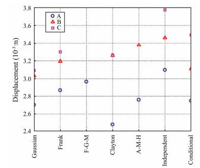
Different design load combinations, as listed in Table 4, were applied to the jacket structure. The dynamic response and maximum displacement of the structure were investigated to ensure the structural safety. All the wave conditions are unidirectional along the x axis. To provide insight into the behavior of the jacket structure under design loads, we analyze the dynamic response of the deck node with the largest response value. The time-displacement (vibration response) curve of platform top points under one given design condition is depicted in Fig.10. Fig.11 shows the maximum displacement of the jacket platform in accordance with various design loads. We observed that the jacket-platform response is at the most extreme when defined using the independent copula model, and the lowest displacement is obtained using a Clayton copula model. Although the Frank copula model is the most suitable distribution to describe the wave data, the determined design loads do not generate more conservative response results than those achieved using the independent copula and conditional distribution model.

5.3 Discussion

The design loads determined using various joint distribution models differ greatly, resulting in different extreme structural response assessments, although the structural extreme response law under different design loads is consistent over the three sets of wave data. In all cases, the Gaussian copula models are in poor agreement with the empirical distribution, with the resulting design loads being low. The design loads obtained using independent copulas are more conservative than those obtained using the other models, which neglect the correlation between environmental variables and result in a higher structural design cost input. The Frank copula class was identified as the most suitable model for the wave data from the three locations, producing a more suitable design load able to ensure the structural design integrity within a certain safety margin. The popular conditional model performs worse than any of the copulas in the goodness-of-fit test. Moreover, the extreme response of the jacket platform obtained using conditional models is larger than those obtained by any of the copulas except the independent copula.

6 Conclusions

This study presents the procedure to determine design loads for an offshore jacket platform using various joint distribution models based on an environmental contour approach. The analytical derivation of the construction of environmental contours is expressed using various classes of copulas, such as Gaussian, Frank, Clayton, AMH, FGM, and independent copula. Moreover, the traditional conditional model for significant wave height and zero-up-crossing period is adopted. The design loads are examined by dynamic response analysis of the jacket structure.

The following conclusions can be drawn from this work:

1) The shapes of environmental contours obtained from various classes of copulas differ greatly for wave data with different degrees of dependency. Thus, excluding the inappropriate copula models according to Kendall's τ is necessary.

2) The goodness-of-fit test indicates that the Frank copula is the most appropriate model for joint distribution of wave data, while the Gaussian copula is in poor agreement with empirical distribution compared with others. Therefore, the Nataf distribution model is unsuitable for the construction of environmental contours in this case. Notably, the suitability of a model for contour construction varies with the origin of the data samples; data from different areas of the sea may be better assessed with other models.

3) The structural extreme response law is concordant across the three datasets (and thus the three sampling areas) used in this study. The environmental contours modeled by the independent copula produce conservative design loads, and the extreme responses obtained using conditional distribution are smaller than those determined by copulas. In addition, the fitting results obtained using conditional models are poorer than those obtained using copulas. Thus, the conditional model is not recommended for the estimation of design loads in those locations.

In summary, this work estimates the design loads for an offshore jacket structure platform based on an environmental contour approach using copulas and the conditional distribution model. This study also assesses the dynamic response of the structure. The results provide a reference for the determination of design loads, which may offer an alternative for determining the design criteria for other offshore structures after complete engineering validation in the future.

Acknowledgements

The study was supported by the National Key Research and Development Program (No. 2016YFC0303401), the National Natural Science Foundation of China (No. 51779236), and the National Natural Science Foundation of China – Shandong Joint Fund Project (No. U1706226).