1 Introduction

The ocean occupies a vast area that is twice as large as that occupied by lands; thus, it has an important contribution to the balance of Earth's ecosystem and provides people with abundant resources. Currently, three main methods are used to explore oceans: deep diving, deep netting, and deep drilling. These enabled us to gain deep insights into oceans. The development of automation technology gradually led to the use of underwater robots as the primary means of underwater operations (Xie et al., 2018; Zhuang et al., 2021; Chen et al., 2022; Duan et al., 2022). Compared with manual operations, underwater robots are known for their high efficiency and low cost. Underwater robots, combined with various sensors and computer vision, can be used to study various topics, namely, aquatic organisms in offshore waters, transmission of information through seabed observation networks in deep seas, and monitoring of underwater organisms and environmental changes through videos and images, which greatly accelerate the development of marine science.

The challenges in underwater image classification include the following: 1) the energy loss of light during the propagation process that reduces its intensity and the uneven spectral propagation that distorts colors with the changes in distance (Mittal et al., 2022); 2) the complex underwater environment that causes underwater images to be susceptible to high noise, low visibility, edge blurring, low contrast, and color deviation. These challenges reduce the visibility of underwater targets and results in blurred underwater images and low contrast. In addition, owing to the differences in water quality, underwater image classification has poor accuracy.

Before the advent of deep learning, underwater image classification tasks often involved human expert-based image annotation and traditional feature-based feature descriptors in the characterization of underwater objects, and features are categorized using classifiers, such as Naive Bayes, ensemble learning, and histograms. Shihavuddin et al. (2013) combined five feature descriptors and four classifiers to investigate six datasets and applied them to the Red Sea dataset to classify coral reef biomes. Mehta et al. (2007) extracted texture features of images, classified coral reef images using support vector machines (SVM) and obtained 95% classification accuracy on a low-quality and small-sample image dataset. In the study of Beijbom et al. (2012), a benchmark dataset of coral reef images was proposed, and image features were by texture and color; training was conducted on the 2008 and 2009 datasets, and an accuracy of 83.1% was achieved on the 2010 dataset, which provides a new solution for the automated ecological analysis of coral reefs. Nadeem et al. (2019) achieved a systematization accuracy of 93.59% on the Eliat Fluorescence Coral dataset by fusing the training results of fluorescence and reflection images. Traditional feature descriptors, such as vein, color, and shape traits, efficiently process images. However, they exhibit poor accuracy because of various underwater image targets, complex environments, and insufficient lighting.

Given their excellent performance in image systematization missions (Simonyan and Zisserman, 2015; Szegedy et al., 2016; Krizhevsky et al., 2017), researchers have quickly applied convolutional neural networks (CNNs to the underwater domain) (Wang et al., 2019; An et al., 2020; Lu et al., 2020; Salman et al., 2020; Irfan et al., 2021). Mahmood et al. (2016) combined VGG (Visual Geometry Group) network extraction and handcrafted features and obtained a classification accuracy of 84.5%. Mahmood et al. (2018) used VGGnet and ResNet in the extraction of common features of coral and noncoral images and realized the automatic annotation of coral population distribution. Compared with that of manual annotation, the computational cost was greatly reduced, and the efficiency was improved, benefiting the long-term detection of marine ecosystems. Prasetyo et al. (2022) combined the low-level features of images with the high-level ones through depthwise separable convolution and improved the fish image classification performance, achieving 98.46% and 97.09% accuracies on the Fish-gres and Fish4Knowledge datasets, respectively. Zhou et al. (2023) proposed a novel ResNet network for the improved classification of fish and invertebrates. Lopez-Vazquez et al. (2023) proposed a convolutional residual network for the classification of marine organisms. Ma et al. (2023) proposed a deep CNN for the classification of underwater sonar images.

Despite the considerable potential of deep learning, end-to-end models cause difficulty in understanding the process of network training and network improvement for specific tasks and model performance. Drawing on the refined processing of each part of a classification task using the traditional classification method, we considered retaining the excellent feature learning capability of a CNN when performing an image classification task while selecting a better classifier to process features.

Traditional classifiers, such as the k-nearest neighbor, SVM, and decision tree, are accompanied by problems, such as the numerous parameters of the model structure that must be adjusted, leading to slow neural network fitting. Pao et al. (1994) proposed a random vector functional link (RVFL) for the random generation of hidden layer biases and input weights of a neural net and used the least squares method to solve the output weights of the hidden layer, which substantially improved the training speed compared with the previous feedforward neural net. Based on a single hidden layer, Tamura and Tateishi (1997) proved that a feedforward neural network with two hidden layers can use (N / 2) + 3 hidden layer nodes to learn the features of N training samples; notably, a single hidden layer feedforward neural network requires N − 1 nodes. Huang (2003) made an additional reduction in the number of required nodes. Meanwhile, Tang et al. (2015) put forward a multilayer coding extreme learning machine (ELM) for the extraction of image features, and it performed better than the existing multilayer perception on multiple classification datasets. Prompted by the multilayer ELM, Shi et al. (2019) proposed a deep RVFL network that adds direct connections from each layer of a network to the original single hidden layer network and includes denoising in autoencoding to obtain better and higher-level feature representations. Experiments by Shi et al. (2019) showed that deep RVFL exhibits an improved performance while requiring fewer hidden layer nodes than ELM. Subsequently, Shi et al. (2019) used the combination of ensemble and deep learning, put forward a general framework for ensemble deep RVFL, and verified its effectiveness using sparse datasets.

This paper proposes a novel underwater image classification model that combines the advantages of RVFLs and deep learning and uses an EfficientnetB0 CNN to abstract traits from underwater images. The RVFL was considered in the classifier, and its network structure was improved. The EfficientnetB0 – two-hidden-layer RVFL (TRVFL) network was used to classify an underwater image dataset.

2 Related Work 2.1 Random Vector Functional Link Network

The RVFL is a relatively simple neural network. Suppose N arbitrary samples (x_i, y_i), where x_i = [x_i1, x_i2, ···, x_in]^T ∈Rⁿ, y_i = [y_i1, y_i2, ···, y_im]^T ∈R^m, and m, n represent the vector's dimensions. The formula for the RVFL network is as follows:

$ \sum\nolimits_{j = 1}^L {{\beta _j}} g({w_j}{X_i} + {b_j}) + \sum\nolimits_{j = L + 1}^{L + d} {{\beta _j}} {X_i}_j = {o_i}, i = 1, 2, \cdot \cdot \cdot, N, $

(1)

where L represents the neuron number, g(x) denotes the function of activation, w_j indicates the input weight, b_j is j-th neuron bias, d corresponds to the input data dimension, and β_j is the output weight. w_j and b_j are randomly generated parameters.

For the minimization of the output error, $ E=\sum_{i=1}^N\left(o_i-y_i\right)$, the following factors must be satisfied:

$ \sum\nolimits_{i = 1}^N {\left\| {{o_i} - {y_i}} \right\|} = 0. $

(2)

The above equation can be directly expressed as follows:

$ \sum\nolimits_{j = 1}^L {{\beta _j}} g({w_j}{X_i} + {b_j}) + \sum\nolimits_{j = L + 1}^{L + d} {{\beta _j}} {X_i}_j = {y_i}, i = 1, 2, \cdot \cdot \cdot, N, $

(3)

Then

$ \boldsymbol H \boldsymbol \beta =\boldsymbol Y, $

(4)

where H represents the hidden layer's output, β denotes the hidden layer's weight, and Y indicates the output. The detailed expressions are as follows:

$\boldsymbol H = {\left[ {\begin{array}{*{20}{c}} {g({w_1}{X_1} + {b_1})}& \cdots &{g({w_L}{X_1} + {b_L})}&{{x_{11}}}& \cdots &{{x_{1n}}} \\ \vdots & \ddots & \vdots & \vdots & \ddots & \vdots \\ {g({w_1}{X_N} + {b_1})}& \cdots &{g({w_L}{X_N} + {b_L})}&{{x_{N1}}}& \cdots &{{x_{Nn}}} \end{array}} \right]_{N \times (L + n)}}, $

(5)

$\boldsymbol \beta = {\left[ {\begin{array}{*{20}{c}} {\beta _1^{\text{T}}} \\ \vdots \\ {\beta _L^{\text{T}}} \\ {\beta _{L + 1}^{\text{T}}} \\ \vdots \\ {\beta _{L + n}^{\text{T}}} \end{array}} \right]_{(L + n) \times m}}, $

(6)

$\boldsymbol Y = \left[ {\begin{array}{*{20}{c}} {y_1^{\text{T}}} \\ \vdots \\ {y_N^{\text{T}}} \end{array}} \right]. $

(7)

The output weight is calculated as $\hat \beta = {H^\dagger }Y$, where H^† represents the inverse matrix.

2.2 EfficientnetB0 Convolutional Neural Network

Efficientnet was used to obtain the backbone network EfficientnetB0 through automatic tuning; the relationship among the width, depth, and resolution of the network was studied, and the best scaling ratio was determined to maintain the network with the highest performance under a given resource condition (Tan and Le, 2019). As for the experimental results on ImageNet, Efficientnet exhibited a higher accuracy while requiring fewer training parameters than other CNNs.

EfficientnetB0 comprises 16 mobile inverted bottleneck convolutions (MBConv), which randomly change the depth of the network with the expansion ratio during the convolution process. As a result, the training speed of the network increases. The Squeeze-and-Excitation Network (SENet) introduced therein features an attention mechanism that helps in the extraction of the main feature information.

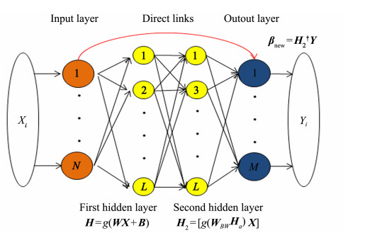
3 Proposed Underwater Image Classification Model 3.1 Two-Hidden-Layer Random Vector Functional Link

The RVFL uses a random assignment to determine input weights and hidden layer biases. In this study, an RVFL network with double hidden layers was proposed. The parameters of the second hidden layer were calculated using a novel method, which resulted in more stable and accurate model outputs. Fig. 1 illustrates the model structure. Parameters other than those of the second layer were the same as those used in the previous generation method, and no changes were made.

The original TRVFL has weight W and bias B at the first hidden layer, and the output of the hidden layer is H = g(WX + B). The weights W and bias B at the second layer are stochastically produced, and the corresponding hidden layer output is H₁ = [g(W₁X + B₁)X]. Finally, the corresponding output weight is obtained by solving the equation $\hat \beta = {H_1}^\dagger Y$. Given the randomly generated parameters of the RVFL, and its performance is affected by the parameters, which results in extensive fluctuations, the improved performance compared with that of the single hidden layer RVFL is not guaranteed. Therefore, in this study, the bias and weight of the second hidden layer were calculated through a new procedure.

The output weight was calculated based on the first hidden layer's output β = [HX]^†Y and the output of the second hidden layer is [H_sX] = Yβ^†. Then, a new augmented matrix W_BW = [B₁ W₁], H_a = [1 H]^T is defined. W_BW is calculated using the following formula:

$ \boldsymbol{W}_{B W}=g^{-1}\left(\boldsymbol{H}_s\right) \boldsymbol{H}_2^{\dagger} . $

(8)

The new second hidden layer output is H₂ = [g(W_BWH_a) X], and its corresponding output weight is $ {\boldsymbol \beta _{{\text{new}}}} = {\boldsymbol H_2}^\dagger \boldsymbol Y $. Finally, the output of TRVFL is f(x) = {g[(W₁g(WX + B) + B₁]X}β_new.

3.2 Underwater Image Classification Model with EfficientnetB0 and TRVFL

The steps for image classification using the EfficientnetB0-TRVFL algorithm are as follows:

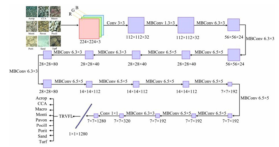
1) For an RGB image, the EfficientnetB0 network requires changing the image size to 224 × 224. After 32 convolutions of 3 × 3 kernels, the size obtained is 112 × 112 × 32.

2) A depth convolution kernel size of 3 × 3 is applied on the 112 × 112 × 32 feature output in step 1. Then, the MB-Conv with an expansion ratio of 1 is used, and the size after convolution becomes 112 × 112 × 16.

3) The depthwise convolution kernel with a size of 3 × 3 MBConv is applied twice on the 112 × 112 × 16 feature out-put in step 2. The expansion ratio is 6, and the postconvolution size has dimensions of 56 × 56 × 24.

4) The depth convolution kernel with a size of 5 × 5 MBConv is applied twice on the 56 × 56 × 24 feature output in step 3. The expansion ratio is 6, and the postconvolution size has dimensions of 28 × 28 × 40.

5) The 28 × 28 × 40 feature output in step 4 undergoes three depth convolutions with a kernel size of 5 × 5. The MBConv has an expansion ratio of 6, and the convolutional size has dimensions of 14 × 14 × 80.

6) The 14 × 14 × 80 feature output in step 5 is subjected to three-time depth convolution with a kernel size of 5 × 5. The MBConv has an expansion ratio of 6, and the size after the convolution is 14 × 14 × 112.

7) The process is conducted four times on the 14 × 14 × 112 feature output from step 6. The depth convolution kernel size, MBConv expansion ratio, and postconvolution size reach 5 × 5, 6, and 7 × 7 × 192, respectively.

8) Depth convolution is performed on the 7 × 7 × 192 feature output in step 7. The depth convolution kernel has a scale of 3 × 3, the expansion ratio is 6, and the size after convolution is 7 × 7 × 320.

9) A 7 × 7 × 320 input image is convolved using 1280 convolution kernels with a size of 1 × 1 to obtain a feature map with dimensions of 7 × 7 × 1280. After obtaining the batch normalization layer, Swish activation function, and global average pooling layer, 1 × 1 × 1280 features are out-putted.

10) The activations() method is used to obtain the output feature matrix, with each sample corresponding to a row with 1280-dimensional feature attributes.

11) The TRVFL classifier is used to replace the softmax classifier to classify features and obtain related results.

Fig. 2 shows the specific process of the EfficientnetB0-TRVFL algorithm model. The trait abstraction method was used with deep learning to process underwater images, and EfficientnetB0 was selected as the CNN structure to obtain a high-performance underwater image classification model. The EfficientnetB0 CNN proposes a unified scaling scale to achieve high efficiency using parameters such as depth, width, and image resolution. Subsequently, the RVFL neural network was improved as a model classifier, and the TRVFL neural network added a hidden layer to the network structure. Simultaneously, to improve the stability of network performance, we proposed a new weight calculation method and replaced the original randomly generated parameter acquisition method. Therefore, classification accuracy can be improved using the TRVFL classifier instead of the softmax classifier to classify features.

4 Experimental Results and Analysis 4.1 Experimental Operating Environment

In this study, six algorithms were compared with the proposed EfficientnetB0-TRVFL algorithm model: Resnet50, VGG16, AlexNet, Googlenet, EfficientnetB0, and EfficientnetB0-RVFL. The laboratory environment involved a computer with a Windows 10 operating system, and MATLAB R2021a software was used.

4.2 Algorithm Parameter Settings

1) Patch size

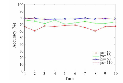
In this study, four different patch sizes were set to abstract trait messages of marked points, and their classification accuracies were compared. For extremely large patch sizes, the surrounding complex environment may disturb the main feature information of the labeled points. Conversely, a small patch size is inadequate to express feature information. However, when the labeling points were located at the boundaries of the two adjacent target types to be classified, the classification results for any patch size were incorrect. Therefore, in this study, patches with four sizes were compared in the MLC 2008 dataset. The overall classification performance was good and very stable when the patch size was 60 pixels (Fig. 3). Therefore, we selected a patch size of 60 pixels for the experiments.

2) Quantity of hidden layer nodes

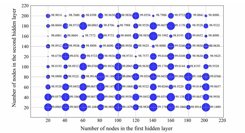
The number of hidden layer nodes is a key factor in neural networks. A very limited number of nodes cause fitting failure of the neural network, resulting in a suboptimal model classification performance. Meanwhile, an extremely high number of nodes will lead to model overfitting, reduce the network classification performance, and waste computing resources. As this study proposed a TRVFL, we set 20 – 200 hidden layer nodes for each layer. The number was incremented by 20, and 100 groups were tested on the Fish-gres dataset. Furthermore, each group of experiments was run ten times, and the average results were obtained. As shown in Fig. 4, the best classification performance was observed when the number of nodes in the second hidden layer was similar to that in the first hidden layer. In addition, given the computing resources, the first and second hidden layers simultaneously contained 80 nodes.

3) Activation function

In addition to data processing, activation functions can be used to enhance the capability of linear classifiers, such as RVFL networks, for better feature representations. The number of hidden nodes was set to 80, and cross-validation of models with different activation functions was used to verify the classification performance. The same type of activation function was used for the two hidden layers. Table 1 shows the outcomes of 10 tests conducted using the EfficientnetB0-TRVFL classification model on the Fishgres dataset with six activation functions. The difference in classification accuracy was insufficient for the six activation functions. In general, when Radbas was used as the activation function, the best classification performance was attained; the average classification result of the Sin activation function was the lowest and significantly lower than those of the other five activation functions. Therefore, Radbas was selected as the activation function of EfficientnetB0-TRVFL for experiments.

4) Other algorithm parameter settings

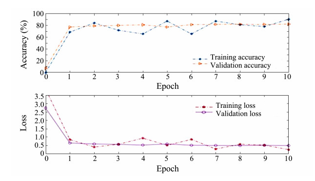
In this study, all the CNN parameters were set uniformly. The iteration round and learning rate were set at 10 and 0.0001, respectively. Verification was performed once per iteration, the batch training scale was set to 64, and the optimizer was set to sgdm. All the CNNs were pretrained, and transfer learning was conducted for dataset classification. For the new fully connected layer, the learning rates of the weights and biases were set to 10, which increased the suitability of the model for underwater image datasets. The TRVFL had the Radbas activation function, and the number of nodes in both hidden layers was set to 80.

4.3 Network Training Process

Fig. 5 shows the classification accuracy and loss of the EfficientnetB0 network during feature extraction from the MLC2008 dataset based on the above algorithm parameters. The upper and lower halves of the figure display the classification accuracy and loss curves, respectively. The abscissa indicates the network for 10 rounds of training, and the different lines denote the classification accuracy and loss of the training and validation sets during the learning process. Fig. 5 also reveals that when EfficientnetB0 was trained with the MLC dataset, the accuracy and loss curves of the training set fluctuated substantially because of the large number of specimens, limited amount of data learned in each iteration process, and uneven distribution and difficulty of various classes of images in the MLC dataset. Overall, the accuracy curves of the training and test sets showed an upward trend, and the loss curve reached good convergence.

4.4 Evaluation Indicators

Four evaluation criteria are typically used to assess the properties of algorithm models in classification tasks: F1-score, recall, precision, and accuracy (Marre et al., 2020; Durden et al., 2021). Regarding multiclassification issues, the MAP can be applied to assess a model's properties, which represents the model's classification capability for all classes. The F1-score is suitable for binary classification tasks. Meanwhile, F1_macro is apt for unbalanced samples and categories of equal importance, which can ensure the classification performance of small sample categories and underwater datasets with unbalanced species. The recall, precision, and F1-score used in the experiments in this study all referred to precision_macro, recall_macro, and F1 _macro, respectively.

The arithmetic expression of evaluation indicators is as follows:

$ {\text{accuracy}} = \frac{{TP + TN}}{{TP + FN + FP + TN}}, $

(9)

$ {\text{precision}} = \frac{{TP}}{{TP + FP}}, $

(10)

$ {\text{recall}} = \frac{{TP}}{{TP + FN}}, $

(11)

$ F{\text{1}} = \frac{{2 \times P \times R}}{{P + R}}, $

(12)

${\text{MAP}} = \frac{{\sum\nolimits_{i = 1}^n {\int_1^0 {p(r){\text{d}}r} } }}{n} , $

(13)

$ precisio{n_{{\text{marco}}}} = \frac{{\sum\nolimits_{i = 1}^n {precisio{n_i}} }}{n} , $

(14)

$ recal{l_{{\text{marco}}}} = \frac{{\sum\nolimits_{i = 1}^n {recal{l_i}} }}{n}, $

(15)

$ F{1_{{\text{macro}}}} = 2 \times \frac{{precisio{n_{{\text{marco}}}} \times recal{l_{{\text{marco}}}}}}{{precisio{n_{{\text{marco}}}} + recal{l_{{\text{marco}}}}}}. $

(16)

where FN indicates that if a sample is positive, then the data will be treated as a negative example. FP denotes the opposite, which means that if a sample is negative, the data will be treated as a positive example. TN means that the data are correctly identified as a negative example. The TP indicates that the data are correctly identified as a positive sample.

4.5 Discussion of Experimental Results 4.5.1 Comparison of experimental results

We confirmed the TRVFL classifier performance by applying EfficientnetB0 to draw the traits of MLC2008, MLC-2009, and Fish-gres datasets and used different classifiers (softmax, TRVFL, and RVFL) to classify and compare the performance evaluation indicators of each algorithm model. Tables 2 – 4 present the experimental results. Each algorithm was run 10 times, where the MLC2008 and Fish-gres datasets were randomly divided by 2:1 and 7:3 per run, respectively. The best outcomes of the algorithms are also listed in the table.

As shown in Tables 2 – 4, the test outcomes of EfficientnetB0 on MLC2008, MLC2009, and Fish-gres datasets were better than those of the other four CNNs. Simultaneously, the RVFL was used to replace the original softmax classification layer in the network, which resulted in a 2% – 3% improvement in the accuracy of EfficientnetB0-RVFL. Compared with the RVFL, after the addition of a hidden layer with a new parameter calculation method, the TRVFL classifier achieved better classification accuracy. For the MLC2008 dataset, the accuracy rate, precision rate, recall rate, F1-score, average accuracy rate, and Cohen's kappa coefficient reached 87.28%, 89.19%, 80.73%, 84.34%, 90.78%, and 0.82, respectively, indicating that the predicted model results were almost identical to the actual classification results. The following results were obtained for the MLC2009 dataset: accuracy rate of 74.06%, precision rate of 78.53%, recall rate of 65.21%, F1-score of 69.59%, average accuracy rate of 82.85%, Cohen's kappa coefficient of 0.61. These values indicate that the predicted outcomes of the model are highly consistent with the actual classification results. For the Fish-gres dataset, the rate of accuracy was 99.59%, the precision rate was 99.55%, the rate of the recall was 99.55%, the F1-score was 99.55%, the average accuracy rate was 99.42%, and Cohen's kappa coefficient of 0.96 indicates that the forecasted outcomes of the algorithm and actual classification results are quite consistent.

According to the experimental results on the three datasets, EfficientnetB0-TRVFL exhibited the best results in terms of various performance evaluation indicators, demonstrating the superiority of its algorithm performance and good generalization.

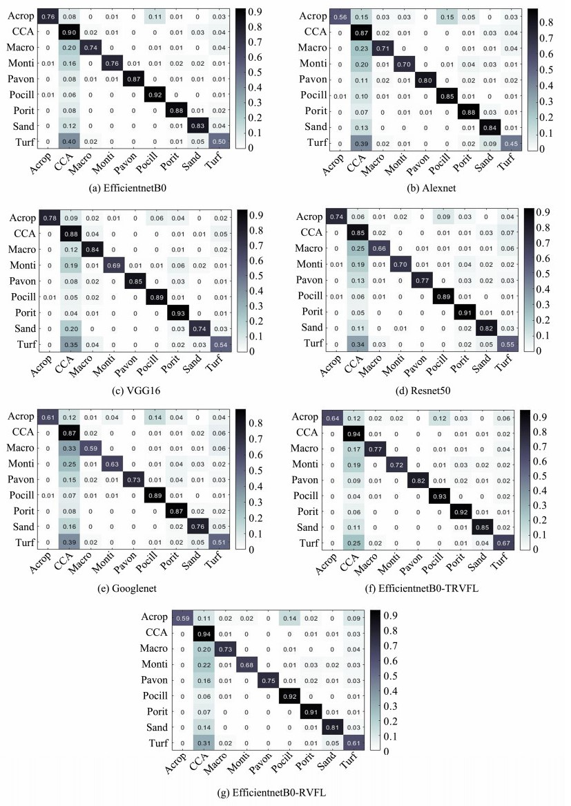
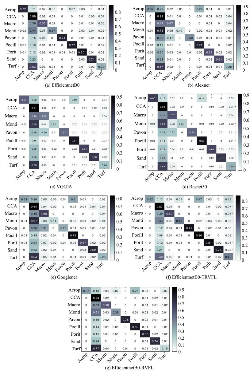
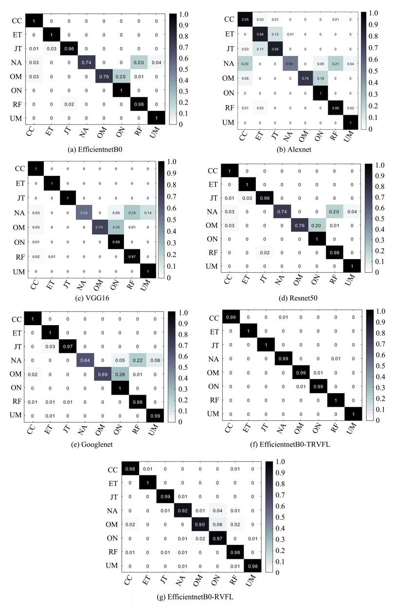
To better illustrate the property improvement of the proposed model compared with traditional classification models, we used five traditional CNNs and EfficientnetB0-RVFL as objects for comparison experiments. Figs. 6 – 8 show the confusion matrix for the proposed algorithm and the other six comparison algorithm models in the MLC2008, MLC2009, and Fish-gres datasets. The row in the figure represents the predicted class, the column denotes the actual class, and the cell with the number 0 indicates that the predicted probability for this cell is less than 0.01. EfficientnetB0-TRVFL obtained excellent classification results for the eight categories in the Fish-gres dataset, whereas for the more challenging MLC2008 and MLC2009 datasets, owing to the interference of the locations of annotation points and complex morphological environment, the confusion between CCA and the other eight categories remained. However, the overall classification accuracy was considerably improved, and almost no confusion was observed in the other categories.

4.5.2 Effectiveness analysis

To demonstrate the advantages of the EfficientnetB0-TRVFL model in underwater image classification tasks, we used the three latest CNNs, namely, Densenet201, Resnet101, and Darknet53, to conduct experiments using the same parameters on the three datasets used in this research. The results of existing methods running on the datasets used in this study were compared. As presented in Table 5, the EfficientnetB0-TRVFL model had an accuracy improvement of 8% – 9% on the MLC2008 dataset, which is 6.48% higher than that of cResFeats (Mahmood et al., 2020); the accuracy of the MLC2009 dataset was increased by 4% – 5%, which is 3.96% higher than that of the combined features (Mahmood et al., 2018) and indicates that the proposed model has the best classification capability for underwater images compared with existing methods.

4.5.3 Stability analysis

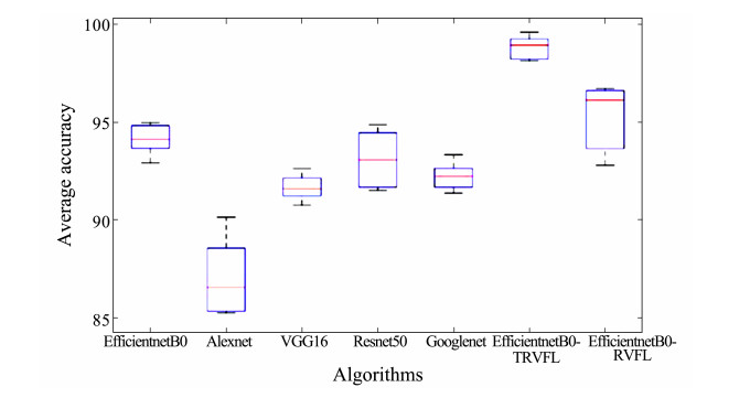
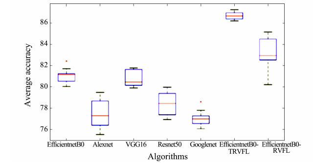
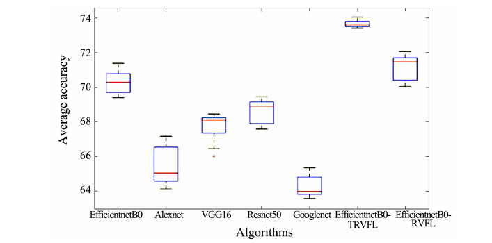
In this study, the stability of the EfficientnetB0-TRVFL algorithm was analyzed through boxplot illustrations. The experimental results were plotted as box plots, which were obtained by running each algorithm 10 times (Figs. 9 – 11). The box positions in the figures represent the overall classification accuracy of each algorithm. The red line denotes the median of outcomes, the red crosses refer to the outliers in data, and the upper and lower boundaries stand for the minimum and maximum values of the results, respectively. The size of the blue box refers to the distribution of results to the top 25% – 75% which also represents the stability of the results. The smaller the box, the better the stability. The distribution of results in the three figures shows that in the MLC2008, MLC2009, and Fish-gres datasets, the proposed EfficientnetB0-TRVFL model attained the best systematization accuracy, and the model put forward by our group is better than most algorithms in terms of stability and has no outliers. In contrast to the Efficient-netB0 network model, the EfficientnetB0-RVFL model owned a certain improvement in accuracy. However, in terms of stability, its performance was superior to that of the softmax classifier owing to the randomness of RVFL parameters.

4.5.4 Significance analysis

The Kolmogorov-Smirnov (KS) test is a nonparametric statistical test. The two-sample KS test was to determine significant differences in the distribution of results. As the KS test requires no data to follow a normal distribution and excludes certain parameters, it is widely used in twosample tests. ${D^*} = {\max _x}\left({\left| {{{\overset{\lower0.5em\hbox{$\smash{\scriptscriptstyle\frown}$}}{F} }_1}(x) - {{\overset{\lower0.5em\hbox{$\smash{\scriptscriptstyle\frown}$}}{F} }_2}(x)} \right|} \right)$represents the distance between the population distribution to which the sample belongs and the given distribution, where F₁(x) and F₂(x) are the distribution functions of the two samples.

The KS test method was used to detect significant differences among algorithms. At the significance level of 0.01, a significant difference was observed when p < 0.01. The opposite was true when p > 0.01. Table 6 lists the test results on the EfficientnetB0-TRVFL algorithm and the compared models. We used bold font to indicate that no evident difference was observed between the algorithms. Remarkable differences were detected between the network model proposed in this study and other models.

5 Conclusions

1) A neural network model with two hidden layers was proposed for the deepening of previous single hidden layers. An unstable network performance was observed due to the randomly generated parameters of the original RVFL model. The TRVFL proposes a new method for the calculation of the parameters in the second hidden layer, which further stabilizes the network and causes no change in the random generation of previous parameters.

2) TRVFL was used to replace the original classifier in the EfficientnetB0 CNN for the classification of underwater images. The algorithm not only uses the advantages of CNN to extract image features but also improves image classification accuracy using the advantages of linear classifiers such as TRVFL.

3) In this study, the advantages of RVFL and traditional CNNs were combined. The EfficientnetB0 model was used to extract underwater features, and the TRVFL model was applied as a classifier to categorize underwater objects. We selected the parameters with the best classification effect as those of the TRVFL network model and used the KS test and boxplots to analyze the significance and stability of the EfficientnetB0-TRVFL model to assess the performance of its algorithm.

4) The size of the dataset image and network parameters were selected through experimental comparison, and the highest classification accuracies (87.28%, 74.06%, and 99.59%) were obtained for the MLC2008, MLC2009, and Fish-gres datasets, respectively. Compared with existing methods, the proposed image classification model has significant performance advantages, high classification accuracy, and good stability.

A deep learning model requires a large amount of data to achieve high accuracy. Therefore, for practical applications of the proposed method, further studies should focus on data enhancement technology of underwater images to overcome the scarcity of training data. Additional studies are also required to ensure the reliability and security of the proposed deep-learning network.

Acknowledgements

We appreciate the support of the National Key R & D Program of China (No. 2022YFC2803903), the Key R & D Program of Zhejiang Province (No. 2021C03013), and the Zhejiang Provincial Natural Science Foundation of China (No. LZ20F020003).