2) Laboratory for Marine Mineral Resources, Qingdao Marine Science and Technology Center, Qingdao 266071, China;
3) College of Underwater Acoustic Engineering, Harbin Engineering University, Harbin 150001, China;
4) Shandong Institute of Geological Survey, Jinan 250014, China
Refraction seismic data obtained through active source exploration using ocean bottom seismometers (OBS) are often used to analyze geological structures (Watremez et al., 2015; Yan et al., 2021). Accurately picking reliable first-arrival travel times is vital for effective refraction data processing (Leung, 2003; Yue et al., 2014). Previous approaches for first-arrival picking chose the position of a sample point according to certain rules (Liao et al., 2011), where the position could only be an integer multiple of the sampling interval. As a result, theoretical errors were observed between the travel time and the picking position, which was especially apparent in low-sampling-frequency OBS data.
Traditionally, manual methods were used for first-arrival picking by identifying variations in waveform and amplitude (Senkaya and Karsli, 2011; Liao et al., 2018; Li et al., 2020). In recent years, researchers have suggested numerous automatic or semiautomatic techniques for first-arrival picking based on time-varying characteristics. Examples include the average energy ratio algorithm for short and long periods (Allen, 1978), the time variance technique between the wave takeoff and the peak (Hatherly, 1982), the energy ratio approach (Coppens, 1985; Baer and Kradolfer, 1987; Earle and Shearer, 1994), the fractal dimension method (Boschetti et al., 1996), the timing attribute technique based on wavelet transform (Tibuleac et al., 2003), the cross-correlation technology (Senkaya and Karsli, 2011, 2014), and the negative-entropy attribute method (Li et al., 2018). These approaches improve the precision and stability of first-arrival picking results from diverse time-varying features. However, these methods are still based on sampling points and do not solve challenges stemming from sampling frequencies.
To improve the precision of first-arrival picking, a novel technique for active source OBS data based on spatial waveform variation characteristics is proposed in this paper. The suggested approach addresses the limitation of a low sampling frequency and achieves results comparable to those of high-sampling-frequency data. The position relationship between the travel time and the picking time from the shot point to the single receiver is analyzed, and the distribution of theoretical errors for all receivers on the survey line is summarized. Because adjacent traces possess similar waveforms and the theoretical errors for the travel time and picking time of adjacent traces are evenly distributed within the sampling interval (Peraldi and Clement, 1972), a label cross-correlation superposition approach is presented here to enhance the frequency of seismic waves and the precision of first-arrival picking. Two methods, namely, the statistical distribution of residuals and the chisquare similarity test, are used to assess the effectiveness of the method. Synthetic data and field data verify that the proposed method is robust and effectively enhances the first-arrival picking accuracy.
2 MethodsIn this section, the theoretical error range based on the relationship between the actual sampling point and the ideal travel time from the shot point to the receiver is investigated. Moreover, the distribution of theoretical errors in the survey line is summarized. Finally, a label cross-correlation superposition approach for adjacent traces is proposed to extract the high-frequency seismic waves.
2.1 Analysis of Theoretical ErrorActive source exploration with OBS that aims to analyze underground geological structures involves engaging sources in seawater; the OBS on the ocean floor receives seismic waves in a particular sampling interval (Huang et al., 2021). The data are generally displayed as a single OBS section, where seismic traces produced by all shot points in the survey line are organized sequentially. In a homogeneous medium, the travel time of the first-arrival wave can be expressed as follows:
| $ t = \frac{{\sqrt {{{\left({{x_s} - {X_r}} \right)}^2} + {{\left({{z_s} - {Z_r}} \right)}^2}} }}{V}, $ | (1) |
where Xr and Zr are the positions of the receiver in the X and Z directions, respectively; xs and zs are the positions of the shot point in the X and Z directions, respectively; and V is the traveling velocity of the seismic wave.
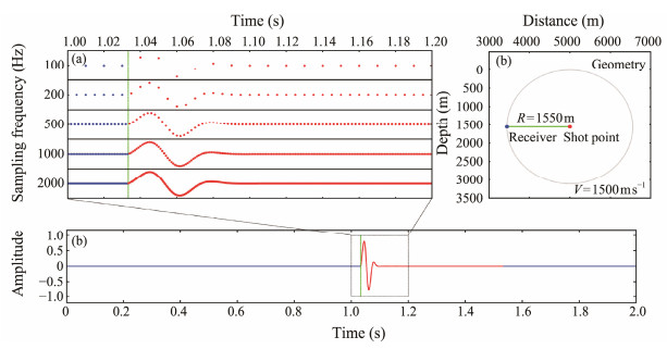
Fig. 1 illustrates an example of the first-arrival picking time error at several sampling frequencies. Fig. 1a presents the digital signals collected using several sampling frequencies (ranging from 100 to 2000 Hz) as dotted lines, which focus on the received waveform in the dashed black rectangle in Fig. 1b, representing the ideal recorded signal with a dominant frequency of 25 Hz. The signal corresponds to the geometry with a fixed offset between the shot point and the receiver in a homogeneous medium, as visualized in Fig. 1c. The amplitude of the solid blue line in Fig. 1b is 0, which indicates the absence of a waveform. The vertical dashed green lines in Figs. 1a and 1b represent the theoretical arrival times of the seismic wave. A theoretical error is observed between the actual sampling point and the theoretical arrival time, and the error increases as the sampling frequency decreases.
|
Fig. 1 Simulation of sampling signal with fixed offset in a homogeneous medium. (a), digital signals logged with several sampling frequencies (100, 200, 500, 1000, and 2000 Hz); (b), signal recorded by the receiver with the vertical dashed green line representing the theoretical arrival time; (c), geometry for the signal in (b) with the dotted gray circle representing a fixed offset from the shot point to the receiver. |
When the sampling frequency is fixed, the theoretical error ∆t (n) of the first-arrival time for multiple shot points in the survey line can be expressed as follows:
| $ \left\{ \begin{array}{l} \Delta t\left(n \right) = M \times {\text{d}}T - t\left(n \right) \hfill \\ t\left(n \right) = \frac{{\sqrt {{{\left({{X_0} + n{\text{d}}X - {X_r}} \right)}^2} + {{\left({{z_s} - {Z_r}} \right)}^2}} }}{V} \hfill \\ \end{array} \right., $ | (2) |
where n is the number of shot points, M is the position of the first-arrival wave in the digital signal, dT is the sampling interval, dX is the shot interval, and X0 is the position of the first shot in the X direction. The range of ∆t (n) can be inferred as [0, dT].
When the shot points and the receiver are on the same horizontal plane, the theoretical error can be expressed as follows:
| $ \Delta t\left(n \right) = M \times {\text{d}}T - \frac{{{X_0} + n{\text{d}}X - {X_r}}}{V}, $ | (3) |
where ∆t (n) is a periodic function of n with the period of VdT/dX, and ∆t (n) is linear with n in a single period. Moreover, n can only be a natural number, so the distribution of the theoretical errors relies on the proportion of the traveling distance per unit time and the shot interval.
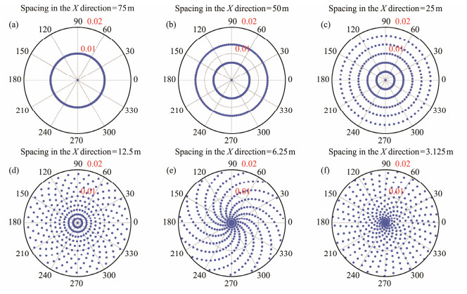
Fig. 2 illustrates the theoretical error distribution of different shot intervals in a homogeneous medium. The survey line comprises 360 shots with a sampling interval of 0.02 s. The receiver is in the first shot position, which is specified in the subgraph's title. The figure is plotted using polar coordinates, where the angle and the radius represent the shot number and the theoretical error, respectively. The theoretical error distribution (Figs. 2a–2c) for several special shot intervals that result in an integer ratio and the periodicity of the error is presented. The theoretical error distribution (Figs. 2d–2f) for several common shot intervals used in offshore seismic exploration, resulting in a noninteger ratio, is also shown. When the receiver and the shot points are on the same horizontal plane, the theoretical errors of the receivers with different shot intervals exhibit overall periodicity despite the diversity of the specific distribution.
|
Fig. 2 Theoretical error distribution of first-arrival picking for different shot intervals in a homogeneous medium. The shot interval is shown in the subgraph's title, the radius represents the value of the theoretical error, and the angle depicts the shot number. |
Varying errors denote the distinct time positions of the seismic wavelet between 0 and the sampling interval. This outcome means that signals with different errors document the seismic wave amplitude at different times, enabling the extraction of high-frequency signals from digital signals with low sampling frequencies. The frequency of the high-frequency signal that can be obtained relies on the proportion of the traveling distance per unit time to the shot interval.
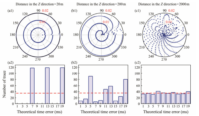
When the shot points and the receivers are not on the same horizontal plane, the theoretical error is not linear with n, and the periodicity is disrupted. The vertical distance between them has a greater effect as it increases. Fig. 3 presents the theoretical error distribution (Figs. 3a1–c1) of the receiver at various depths with shot intervals of 50 m in a homogeneous medium, along with the corresponding trace number of errors in small time windows of 2 ms (Figs. 3a2–c2). The depth of the receiver influences the periodicity of the theoretical error, with a greater effect observed at near offsets. As the depth increases, the influence range gradually grows, and the number of theoretical errors in small time windows becomes closer to the average. Active source OBS acquisition utilizes an air-gun array as its source, and OBS is deployed to receive seismic waves on the seafloor. Active source OBS acquisition overcomes the limitations of the offset range in traditional stream acquisition (Liu, 2015). Only a few of the early arrivals are direct waves, whereas the rest are reflections through the geological layers. An improved bending approach is used here to compute the first-arrival time and examine the theoretical error (Koulakov et al., 2010). Fig. 4 shows the theoretical error of active source OBS data in layered seafloor media. The theoretical error is irregularly spread within the sampling interval, but the trace numbers of theoretical errors in small time windows are uniform.
|
Fig. 3 Theoretical error distribution at different receiving depths in a homogeneous medium. (a1)–(c1), theoretical error distribution in polar coordinates. The depth of the receiver is specified in the subgraph's title, the radius represents the theoretical error, and the angle depicts the trace number. (a2)–(c2), corresponding trace number of errors in small time windows. The abscissa is the theoretical error (the unit is ms), the width of each bin is 2 ms, and the dashed red line is the average number of traces. |

|
Fig. 4 Theoretical error of active source OBS under layered submarine media. (a), velocity field and geometry; (b), theoretical error distribution in polar coordinates; (c), corresponding trace number of errors in small time windows. |
In addition, the velocity of seismic waves in seawater varies, the shot interval is inconsistent, and the OBS location may diverge from the deployment position. These actual conditions can also influence the travel time of the first-arrival wave and cause uncertainty in the theoretical error. Thus, the theoretical errors of the first-arrival waves across the entire OBS section are dispersed within the sampling interval range, and the trace number of errors in small time windows is evenly spread. Low-frequency data, which record seismic wave values at different times, can be used to obtain high-frequency waveforms from multiple traces. Considering the complexity of the actual signal and the attenuation of seismic waves, it is used only to enhance the picking precision of the first-arrival wave with small waveform variations.
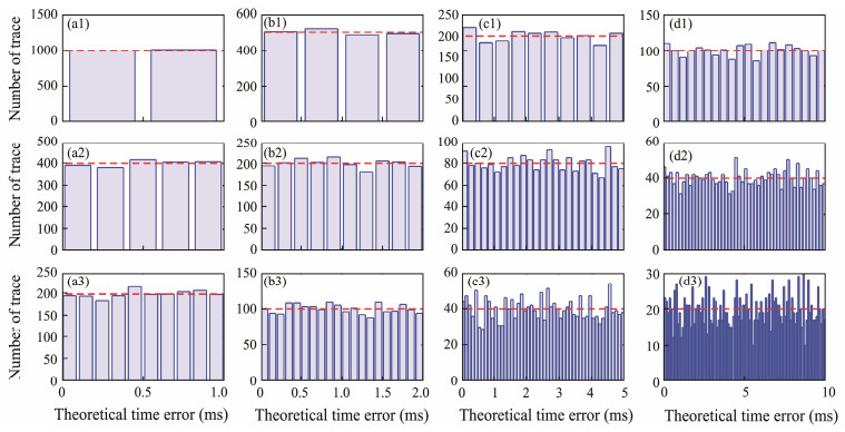
The number of shot points on a survey line is restricted, and interference waves are not avoided in the record. Therefore, the frequency of seismic waves cannot be infinitely increased. The appropriate frequency for extracting seismic waves should be chosen based on the distribution of theoretical errors. Fig. 5 illustrates the trace number of theoretical errors for several sampling frequencies of 1000, 500, 200, and 100 Hz in three time windows of 0.5, 0.2, and 0.1 ms. Within the range of the theoretical error, the fewer the time windows, the greater the average trace number of the errors in each window. In low-frequency data, a smaller time window is chosen; hence, the trace number of errors is not uniform. When extracting high-frequency seismic waves, the trace number of theoretical errors in each time window must be uniform; that is, the proportion of each error point is the same.
|
Fig. 5 Trace numbers of theoretical errors with varied sampling frequencies (1000, 500, 200, and 100 Hz) in three small time windows (0.5, 0.2, and 0.1 ms, respectively). The abscissa is the theoretical error (the unit is ms), and the dashed red line depicts the average number of traces in small time windows. |
First-arrival wave picking is split into three key steps. First, the initial position of the first-arrival wave is picked up by the existing picking technique, such as the energy ratio method (Sabbione and Velis, 2010; Liu et al., 2022), and the window is chosen based on the initial position. Then, the high-frequency seismic waves are obtained by using the label cross-correlation superposition method. Finally, according to the initial picking position, the seismic waves are inverted and flattened, and the current method is used to obtain the first-arrival wave again.
In this section, the approach for extracting high-frequency seismic waves from low-frequency data of adjacent traces is mainly introduced. The waveforms of adjacent traces in the seismic section are similar, especially in the same wave group (Liu et al., 2021). The cross-correlation technique (CCT) can showcase their similarity at different times and lower the influence of random noise. In the cross-correlation, the relative time shift of two signals moves in accordance with the sampling interval. Theoretically, the cross-correlation between adjacent traces within a small window range centered on the arrival time of the first-arrival wave has a maximum value at zero-time delay. However, the precision of first-arrival picking is restricted because seismic waves do not always spread as an integer multiple of the sampling interval.
To acquire a higher resolution correlation coefficient, the low-frequency data were interpolated to create the high-frequency data. The interpolated data were marked as 0, whereas the original data were marked as 1. Next, multiple traces centered on the reference trace were selected, and their cross-correlation coefficients with the reference trace were computed. The deviation between the maximum and intermediate positions was recorded as the time delay between the two traces. Finally, the average of adjacent traces corrected by the time delay was quantified and taken as the high-frequency seismic waves.
If the original sampling frequency of seismic wave x(n)n∈[1, 2, ···, N] is F1, it was interpolated to achieve a new sampling frequency of K × F1, and the interpolated data were marked as follows:
| $ x\left(m \right) = {x^*}\left(m \right) \times s\left(m \right), {\kern 1pt} {\kern 1pt} {\kern 1pt} m \in \left[ {1, 2, \cdot \cdot \cdot, K\left({N - 1} \right) + 1} \right], $ | (4) |
where N is the number of sample points, x*(m) is the interpolated high-frequency data, and s(m) is a marking function that can be represented as follows:
| $ s\left(m \right) = \left\{ {\begin{array}{*{20}{c}} {1, {\kern 1pt} {\kern 1pt} {\kern 1pt} m = 1, K + 1, \cdot \cdot \cdot, K\left({N - 1} \right) + 1} \\ {0, {\kern 1pt} {\kern 1pt} {\kern 1pt} m \ne 1, K + 1, \cdot \cdot \cdot, K\left({N - 1} \right) + 1} \end{array}} \right.. $ | (5) |
M is the number of interpolated sample points. The cross-correlation coefficient (Costa, 2021) of adjacent traces can be expressed as follows:
| $ {c_{xy}}\left(i \right) = \mathop \sum \limits_{j = 1}^M x_1^*\left(j \right)x_2^*\left({i + j - M} \right), {\kern 1pt} {\kern 1pt} {\kern 1pt} i = 1, 2, \cdot \cdot \cdot, 2M - 1 . $ | (6) |
The deviation between the position of the local maximum and the intermediate position of the cross-correlation coefficient stands for the relative time delay parameter of the two traces.
Owing to the absorption of seawater and strata, seismic waveforms can become complex. Therefore, a specific amount of adjacent trace data with similar characteristics must be stacked to acquire high-frequency seismic waves in practical data processing. The data from adjacent traces are denoted as x1, x2, ···, xC, and the high frequency of seismic waves can be stated as follows:
| $ \bar x = \mathop \sum \limits_{i = 1}^C x_i^*{s_i}\left({{\tau _i}} \right)/\mathop \sum \limits_{i = 1}^C {s_i}\left({{\tau _i}} \right), $ | (7) |
where τi is the relative time delay parameter derived from the cross-correlation coefficient of each trace. The denominator is a stacking array of corresponding marking functions, and each element is greater than 1.
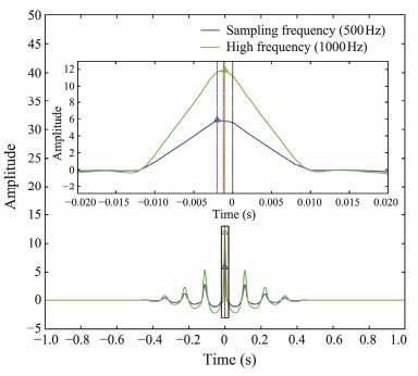
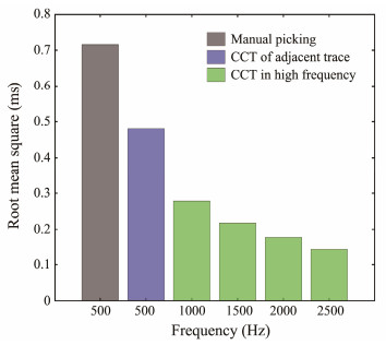
Simulation data were utilized to demonstrate the effectiveness of this approach. Fig. 6 displays the cross-correlation results of the high- and low-frequency data in adjacent traces. The moving step of high-frequency data was smaller than that of low-frequency data, causing a smoo-ther cross-correlation curve (green line). The time delay parameters acquired from the cross-correlation results of the interpolated high-frequency data (the dashed blue line) were closer to the theoretical position (the dashed red line) than those of the low-frequency sampled data (the dashed green line). To demonstrate the influence of different interpolation frequencies on the time delay parameters, the root mean square of the difference between the calculated and theoretical positions of all traces was computed, as shown in Fig. 7. The low-frequency sampled data exhibited a large theoretical error (gray rectangle), which can be decreased through the adjacency CCT (blue rectangle). More importantly, this approach can further decrease the theoretical error by extracting high-frequency data, whose error decreases gradually with the increase of frequency (green rectangles).
|
Fig. 6 Cross-correlation results of high- and low-frequency data in adjacent traces. The blue and green lines correspond to the sampling low-frequency results and the interpolated high-frequency results, respectively. The dashed black line is the middle position, the dashed red line is the position that must be adjusted theoretically, and the dashed blue line and the dashed green line correspond to the adjustment position obtained by the cross-correlation results of high and low frequencies, respectively. The top subgraph is a larger display of the black rectangle in the bottom subgraph. |
|
Fig. 7 Root mean square of the time delay parameters in all traces for different frequencies. |
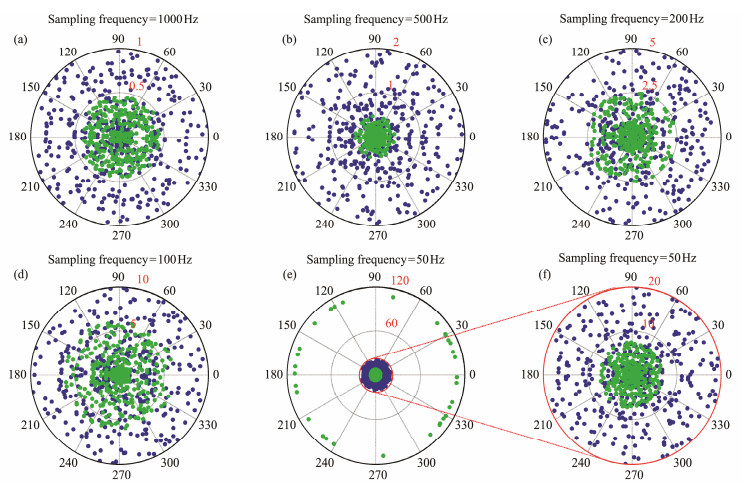
Fig. 8 compares the theoretical errors before and after the extraction of high-frequency data at various sampling frequencies. The sampling frequency decreased from 1000 Hz to 50 Hz, and the high-frequency data of 2000 Hz were collected using the above method. Afterward, the residual error between the theoretical position and the first-arrival picking position was determined. The seismic wavelet was generated using the air-gun wavelet simulation method based on the van der Waals equation, and the first notch was set to 94 Hz (Xing et al., 2022). When the sampling frequency was greater than the first notch (Figs. 8a–8d), this method effectively improved the precision of the first-arrival picking. For most traces, the precision of the first-arrival picking was improved when the sampling frequency was less than that of the first notch (Fig. 8f). However, some abnormal traces with unusual values of around 110 ms (Fig. 8e), which was equal to the vibration period of the seismic wavelet, were observed.
|
Fig. 8 Comparison of theoretical errors before and after extracting high-frequency data at different sampling frequencies. The blue and green dots correspond to the sampling low-frequency data and the extracted high-frequency data, respectively. |
In this section, synthetic data were used to assess the applicability of the proposed approach. The first arrivals of high- and low-frequency data were picked up, which high-lighted the effect of low sampling frequency on the picking results. An appropriate window was chosen to extract the first-arrival wave with the initial position picking in the low-frequency sampled data as the center. Then, a specific number of adjacent traces were chosen to collect high-frequency seismic waves using the proposed method. Finally, the seismic wave was inverted and flattened according to the initial position, and the first-arrival wave was obtained. The results of the first-arrival picking were assessed by the distribution and various residual statistics (maximum, minimum, average, and median) between the picking result and the theoretical arrival time. The chi-square similarity test (Chen and Chen, 2011) was used to assess the overall consistency, where P is the reliability, and an H less than 0.05 indicates the similarity of the results.
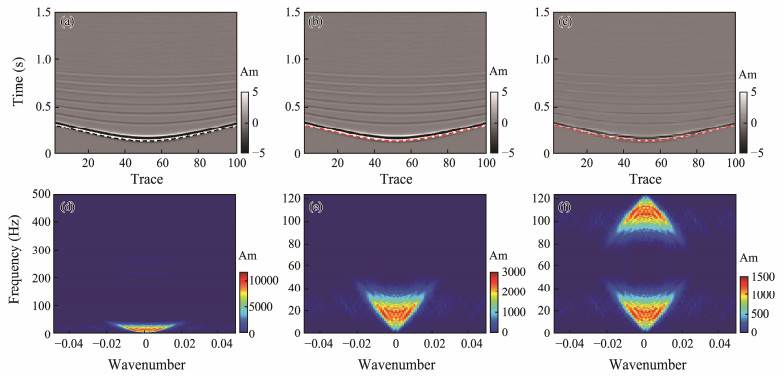
In the synthetic tests, the first arrival of noiseless data with a sampling frequency of 1000 Hz was taken as the theoretical arrival time (Fig. 9a, dashed black line). Then, the data with a sampling frequency of 250 Hz were resampled as high-frequency data (Fig. 9b), and half of the data were regularly assigned to 0 in the time direction to recreate the low-frequency data (Fig. 9c). The modified energy ratio approach (Sabbione and Velis, 2010) was used to de termine their first-arrival time. Fig. 9 presents the waveform, and the first-arrival picking results, and the final parameters are shown in Table 1. In the high-frequency sampled data (Fig. 9b), the range of the residuals was between 1 and 5 ms, the average was 3.099 ms, and the median was 3 ms. However, in the low-frequency sampled data (Fig. 9c), the range of residuals increased to 0 – 9 ms, the average was 4.762 ms, and the median was 5 ms. The chi-square similarity test result decreased from 0.94533 to 0.91644, exhibiting unsatisfactory picking performance at low sampling frequencies. Figs. 9d–9f show the F-K spectrum corresponding to the data with varied sampling frequencies. A frequency folding event can be seen in the spectrum of the low-frequency sampled data (Fig. 9f).
|
Fig. 9 Waveforms of the simulated data at various frequencies. (a), 1000 Hz; (b), 250 Hz; and (c), 125 Hz. The results of the first-arrival picking are plotted as dashed lines on the waveforms. (d)–(f) corresponding F-K spectrum. Am, amplitude. |
|
|
Table 1 Evaluation parameters in the synthetic tests |
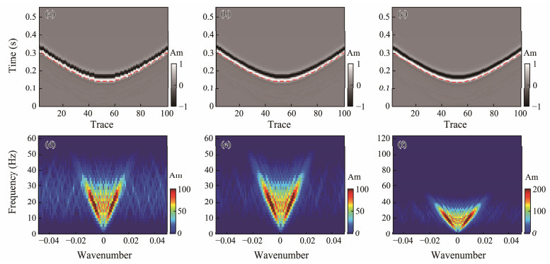
Fig. 10a presents the waveform at the simulated low frequency within a time window of 0.2 s. The result of the first-arrival wave was drawn above it using a dashed red line. Fig. 10b shows the first-arrival positions of the seismic waves extracted by the CCT from low-frequency sampled data. The chi-square similarity test result increased to 0.92045, as shown in Table 1. However, no remarkable enhancement in the distribution and statistics of the residual error was observed, which indicates that the result can only be improved to a certain extent. Fig. 10c presents the seismic waveform and the outcomes of the first arrival using the proposed approach. The chi-square similarity test result increased to 0.94258, as shown in Table 1, and the distribution and statistics of the residual error were reduced, which did not differ much from the picking result of the high-frequency data, as shown in Fig. 9b. This technique can achieve the same first-arrival picking precision as the high-frequency sampling data. Figs. 10d–10f display the F-K spectrum of the data. By performing cross-correlation extraction of the adjacent traces, the interference components on both sides of the seismic wave spectrum in the wave-number direction were suppressed, hence improving the signal-to-noise ratio, as shown in Fig. 10f.
|
Fig. 10 Waveforms of the simulated data. (a), low-frequency sampled data of 125 Hz; (b), CCT of adjacent traces at the frequency of 125 Hz; and (c), the proposed method at the frequency of 250 Hz. The results of the first-arrival picking are plotted as dashed lines on the waveforms. (d)–(f) corresponding F-K spectra. Am, amplitude. |
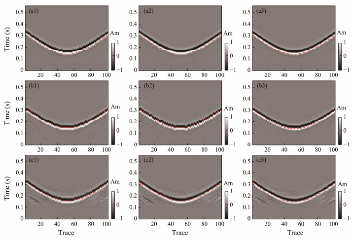
To evaluate the robustness of our proposed method, 1%, 5%, and 10% Gaussian random noise were added to the synthetic data, and the first-arrival wave was obtained using the same method (Fig. 11 and Table 2). At several noise levels, traditional CCT at low frequencies enhanced the chi-square similarity test outcome but failed to lower the distribution range of the residual error. By contrast, the proposed technique not only enhanced the overall similarity coefficient but also reduced the residual error distribution. However, the results of the chi-square similarity test gradually decreased with increasing noise levels. This occurs because, when handling data with high noise levels using the energy ratio method, the window length and thres-hold needed to be increased to derive stable picking results, leading to an overall hysteresis in the picking position.
|
Fig. 11 Waveform and first-arrival picking results of seismic waves with different levels of random noise. The results of the first-arrival picking are plotted as dashed lines on the waveforms. (a1), initial position, 1% noise; (a2), CCT of adjacent trace, 1% noise; (a3), proposed method, 1% noise; (b1), initial position, 5% noise; (b2), CCT of adjacent trace, 5% noise; (b3), proposed method, 5% noise; (c1), initial position, 10% noise; (c2), CCT of adjacent trace, 10% noise; and (c3), proposed method, 10% noise. Am, amplitude. |
|
|
Table 2 Evaluation parameters at different noise levels |
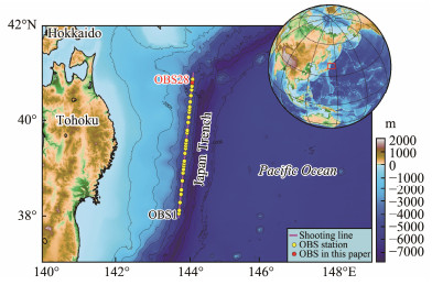
In this section, the OBS data acquired with a low sampling frequency were selected to validate the proposed method. Fig. 12 shows the data obtained in the west of the Japan Trench with an air-gun array of 100 L (Azuma et al., 2018). The data set (Fig. 13a) of OBS28 with a sampling frequency of 128 Hz was selected. The data preprocessing involved band-pass filtering and trace equalization.
|
Fig. 12 Map of the study area. The magenta line is the shooting line, the yellow circles denote the OBS station in the Japan Trench, and the red circle denotes the OBS used in this paper. |
|
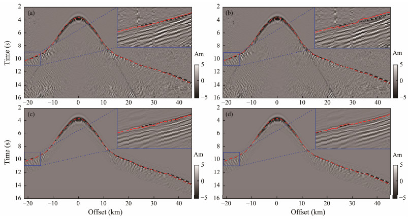
Fig. 13 Waveforms and picking results of first arrival as dashed lines in the field data validation. (a), original sampling frequency data of 128 Hz; (b), low-frequency sampled data of 64 Hz; (c), CCT of adjacent traces with the frequency of 64 Hz; (d), proposed method with the frequency of 128 Hz. Am, amplitude. |
To quantify the effectiveness of the proposed method, 128 Hz was set as the high sampling frequency, and the first-arrival wave was manually picked as the correct travel time (Fig. 13a, dashed black line). Then, an automated technique was used to pick the first-arrival wave (Fig. 13a, red line). To replicate the low-frequency data, half of the data in the time direction were regularly deleted, and the same method was used to pick the first-arrival wave (Fig. 13b). The corresponding evaluation parameters are presented in Table 3. After re-sampling, the distribution range and statistics of the residual error increased, revealing decreased picking precision. Afterward, a proper window was chosen to obtain the first-arrival wave with the initial picking position as the center in the low-frequency data. The CCT at low frequencies (Fig. 13c) and our proposed method (Fig. 13d) were used to pick the first-arrival wave. The former did not substantially enhance the distribution and statistics of the residual error, whereas the latter achieved outcomes similar to those acquired directly in the high-frequency data.
|
|
Table 3 Evaluation parameters in the field data validation |
In addition, the waveform recording showed that the proposed approach enhanced the signal-to-noise ratio of the data, improved the continuity of the first-arrival waves, and achieved high-precision picking outcomes.
5 ConclusionsIn this paper, an approach to pick the first-arrival wave of OBS data based on spatial waveform variation characteristics is proposed. The high-frequency seismic waves were extracted from the low-frequency sampled seismic waves of the adjacent traces, and the first-arrival wave was obtained. The proposed method addressed the constraint of the sampling frequency and increased the picking precision of the first-arrival wave. The synthetic data demonstrated the effectiveness of the proposed approach. The proposed method was then applied to the data of active source exploration with OBS. The following conclusions are drawn.
1) The theoretical errors of the first-arrival waves picking in the OBS data were spread within the range of the sampling interval, and the number of errors in the small time windows was evenly dispersed across the traces.
2) The high-frequency seismic waves from adjacent traces with low sampling frequency were extracted by utilizing the spatial waveform variation characteristics. This method improved the frequency content of the data and consequently strengthened the precision of picking the first-arrival waves.
3) Synthetic data exhibited that the proposed approach can effectively increase the precision of first-arrival picking at diverse noise levels. Moreover, the field data achieved picking outcomes with precision equivalent to that of the high-sampling-frequency data.
4) The precision of first-arrival picking was innately constrained in the practical seismic data owing to the finite number of shot points on a survey line and the existence of unavoidable noise. Therefore, the precision of first-arrival picking cannot be improved infinitely.
AcknowledgementsThis work was supported by the Major Research Plan on West-Pacific Earth System Multispheric Interactions (Nos. 91858215, 91958206), the National Natural Science Foundation of China (NSFC) Shiptime Sharing Project (No. 41949581), and the Key Research and Development Program of Shandong Province (No. 2019GHY112019).
Allen, R. V., 1978. Automatic earthquake recognition and timing from single traces. Bulletin of the Seismological Society of America, 68(5): 1521-1532. DOI:10.1785/BSSA0680051521 (  0) 0) |
Azuma, R., Hino, R., Ohta, Y., Mochizuki, K., Uehira, K., Murai, Y., et al., 2018. Along-arc heterogeneity of the seismic structure around a large coseismic shallow slip area of the 2011 Tohoku-Oki earthquake: 2-D Vp structural estimation through an air gun-ocean bottom seismometer experiment in the Japan Trench subduction zone. Journal of Geophysical Research: Solid Earth, 123: 5249-5264. DOI:10.1029/2017JB015361 (  0) 0) |
Baer, M., and Kradolfer, U., 1987. An automatic phase picker for local and teleseismic events. Bulletin of the Seismological Society of America, 77(4): 1437-1445. DOI:10.1785/BSSA0770041437 (  0) 0) |
Boschetti, F., Dentith, M. D., and List, R. D., 1996. A fractal-based algorithm for detecting first arrivals on seismic traces. Geophysics, 61(4): 1095-1102. DOI:10.1190/1.1444030 (  0) 0) |
Chen, Y. T., and Chen, M. C., 2011. Using chi-square statistics to measure similarities for text categorization. Expert Systems with Applications, 38(4): 3085-3090. DOI:10.1016/j.eswa.2010.08.100 (  0) 0) |
Coppens, F., 1985. First arrival picking on common-offset trace collections for automatic estimation of static corrections. Geophysical Prospecting, 33(8): 1212-1231. DOI:10.1111/j.1365-2478.1985.tb01360.x (  0) 0) |
Costa, L. D. F., 2021. Comparing cross correlation-based similarities. Arxiv Preprint: 2111.08513, https://doi.org/10.48550/arXiv.2111.08513.
(  0) 0) |
Earle, P. S., and Shearer, P. M., 1994. Characterization of global seismograms using an automatic-picking algorithm. Bulletin of the Seismological Society of America, 84(2): 366-376. DOI:10.1785/BSSA0840020366 (  0) 0) |
Hatherly, P. J., 1982. A computer method for determining seismic first arrival times. Geophysics, 47(10): 1431-1436. DOI:10.1190/1.1441291 (  0) 0) |
Huang, H., Klingelhoefer, F., Qiu, X., Li, Y., and Wang, P., 2021. Seismic imaging of an intracrustal deformation in the northwestern margin of the South China Sea: The role of a ductile layer in the crust. Tectonics, 40: e2020TC006260. DOI:10.1029/2020TC006260 (  0) 0) |
Koulakov, I., Stupina, T., and Kopp, H., 2010. Creating realistic models based on combined forward modeling and tomographic inversion of seismic profiling data. Geophysics, 75(3): B115-B136. DOI:10.1190/1.3427637 (  0) 0) |
Leung, T. M., 2003. Controls of traveltime data and problems of the generalized reciprocal method. Geophysics, 68(5): 1626-1632. DOI:10.1190/1.1620636 (  0) 0) |
Li, C., Liu, J. X., Liao, J. P., and Hursthouse, A., 2020. 2D high-resolution crosswell seismic traveltime tomography. Journal of Environmental & Engineering Geophysics, 25(1): 47-53. DOI:10.2113/JEEG19-003 (  0) 0) |
Li, Y., Ni, Z., and Tian, Y., 2018. Arrival-time picking method based on approximate negentropy for microseismic data. Journal of Applied Geophysics, 152: 100-109. DOI:10.1016/j.jappgeo.2018.03.012 (  0) 0) |
Liao, J. P., Guo, Z. W., Liu, H. X., Dai, S. X., Zhao, Y. L., Wang, L. X., et al., 2018. Application of frequency-dependent travel-time tomography to 2D crosswell seismic field data. Journal of Environmental & Engineering Geophysics, 22(4): 421-426. DOI:10.2113/JEEG22.4.421 (  0) 0) |
Liao, Q., Kouri, D., Nanda, D., and Castagna, J., 2011. Automatic first break detection by spectral decomposition using minimum uncertainty wavelets. SEG Technical Program Expanded Abstract 2011. Society of Exploration Geophysicists, 1627-1631, https://doi.org/10.1190/1.3627515.
(  0) 0) |
Liu, C., 2015. Study on wide-angle seismic exploration of deep tectonic in the South Yellow Sea. PhD thesis. Ocean University of China.
(  0) 0) |
Liu, H. W., Liu, H. H., Xing, L., and Li, Q. Q., 2022. A new method for OBS relocation using direct water-wave arrival times from a shooting line and accurate bathymetric data. Marine Geophysical Research, 43(2): 20. DOI:10.1007/s11001-022-09482-0 (  0) 0) |
Liu, Q., Fu, L., and Zhang, M., 2021. Deep-seismic-prior-based reconstruction of seismic data using convolutional neural networks. Geophysics, 86(2): V131-V142. DOI:10.1190/geo2019-0570.1 (  0) 0) |
Peraldi, R., and Clement, A., 1972. Digital processing of refraction data study of first arrivals. Geophysical Prospecting, 20(3): 529-548. DOI:10.1111/j.1365-2478.1972.tb00653.x (  0) 0) |
Sabbione, J. I., and Velis, D., 2010. Automatic first-breaks picking: New strategies and algorithms. Geophysics, 75(4): V67-V76. DOI:10.1190/1.3463703 (  0) 0) |
Senkaya, M., and Karsli, H., 2011. First arrival picking in seismic refraction data by cross-corelation technique. 6th Congress of the Balkan Geophysical Society. European Association of Geoscientists & Engineers, Budapest, cp-262-00022.
(  0) 0) |
Senkaya, M., and Karsli, H., 2014. A semi-automatic approach to identify first arrival time: The cross-correlation technique (CCT). Earth Sciences Research Journal, 18(2): 107-113. DOI:10.15446/esrj.v18n2.35887 (  0) 0) |
Tibuleac, I. M., Herrin, E. T., Britton, J. M., Shumway, R., and Rosca, A. C., 2003. Automatic secondary seismic phase picking using wavelet transforms. 25th Seismic Research Review – Nuclear Explosion Monitoring: Building the Knowledge Base. Tuscon, 352-359.
(  0) 0) |
Watremez, L., Helen Lau, K. W., Nedimović, M. R., and Louden, K. E., 2015. Traveltime tomography of a dense wide-angle profile across Orphan Basin. Geophysics, 80(3): B69-B82. DOI:10.1190/geo2014-0377.1 (  0) 0) |
Xing, L., Lin, H. R., Zhang, D., Li, Q. Q., Zhou, H. W., and Liu, H. S., 2022. Facial characteristics of air gun array wavelets in the time and frequency domain under real conditions. Journal of Applied Geophysics, 199: 104591. DOI:10.1016/j.jappgeo.2022.104591 (  0) 0) |
Yan, Y. N., Liao, J. P., Yu, J. H., Chen, C. L., Zhong, G. J., Wang, Y. L., et al., 2021. Velocity structure revealing a likely mud volcano off the Dongsha Island, the northern South China Sea. Energies, 15(1): 195. DOI:10.3390/en15010195 (  0) 0) |
Yue, B. B., Peng, Z., and Zhang, Q., 2014. Seismic wavelet estimation using covariation approach. IEEE Transactions on Geoscience and Remote Sensing, 52(12): 7495-7503. DOI:10.1109/TGRS.2014.2313116 (  0) 0) |
 2024, Vol. 23


