Ⅰ、DIAGNOSTIC UNCERTAINTY

We always face diagnostic uncertainty. Decision making, by means of diagnostic tests, is a major task to clinicians, especially in critical patients. Take an example. A man comes with chest pain at 2 am.The gold standard of cardiac catheterization to see if there is any occlusion of coronary arteries, remains the best option. However it is invasive. Cardiologists and laboratory support may not be available. But minutes count. We may want to have a reliable diagnostic test to rule in or rule out myocardial infarct.

Diagnostic test studies differs from Clinical Prediction Rule studies.Clinical Prediction Rule uses the rule to predict outcome, instead of diagnosing the outcome. For diagnostic test study, the test result may be dichotomous, or multi-level (continuous). For dichotomous test, such as bedside ultrasound to diagnose pneumonia, we may construct a 2×2 table for calculation. There is only a single set of sensitivity and specificity.For continuous data, e.g.amylase level for pancreatitis, and, troponin level in myocardial infarct, we can have multi-level cuts. We can construct a Receiver Operating Characteristic (ROC) Curve for multi-level cuts.

Ⅱ、CLINICAL DIRECTNESS

Appraising diagnostic test article starts with the population P, then the diagnostic test concerned (viewed as exposure E) & then the outcome O (the disease or condition the test is used to diagnose) =>PEOs.

Ⅲ、VALIDITY 1. Gold standard that is acceptable, independent and done on all tested subjects

To measure the diagnostic accuracy of a test, we need to compare its result with a gold standard.This gold standard is an acceptable one to confirm the presence or absence of a disease.Theoretically, it is 100% sensitive and 100% specific.Gold standard should be interpreted independently from diagnostic test. Blinding may be needed to avoid bias. And all subjects being tested, must be verified by gold standard.

2. Risks of bias:Spectrum bias and Verification bias

Spectrum Bias:An unrecognized (but probably very real) problem is that of spectrum bias. This is the phenomenon of the sensitivity and/or specificity of a test varying with different populations tested - populations that may vary in sex ratio, age, or severity of disease. Yet subgroup heterogeneity is not a bias if appropriate analyses are conducted. The sensitivity, specificity and likelihood ratios can be stratified, according to the subgroups. We should address the heterogeneity in the analysis and application.

If we recruit subjects with no disease and subjects with severe disease, we expect the accuracy of the diagnostic test will be high. Spectrum bias occur. Sensitivity and specificity results may be unstable if there is spectrum bias. Hence we should include subjects with a spectrum of severity, that is, subjects with no disease, and, subjects with mild, moderate and severe disease together.

Verification bias:This occurs when patients with negative test results are not evaluated with the gold standard test. A study selectively includes patients for disease verification by gold standard testing, based on positive results of preliminary testing, or the study test itself. For example, if Coronary angiogram applies on subjects with raised troponin level but not the others, verification bias results. To avoid this, a study should include consecutive patients at risk for a particular disease, and not only a subset who undergo definitive testing. So to speak, all subjects should be verified by gold standard.

Diagnostic test should also be independent from gold standard, and vice versa.Take an example of myocardial infarct. According to World Health Organization (WHO) criteria, 2 out of 3 having raised cardiac enzymes, chest pain and abnormal ECG, can be identified as gold standard for myocardia infarct. Problems may arise when we choose Troponin as diagnostic test, as well as, one of criteria of gold standard under WHO.

Ⅳ、RESULTS

Dichotomous data using a 2×2 table:

Prevalence: The proportion of a population having a particular condition or characteristic: e.g. the percentage of people in a city with a particular disease = (a+c)/(a+b+c+d). You can refer this as 'pre-test probability'.

Accuracy= (a+d)/(a+b+c+d) = (TP and TN)/all

Sensitivity= True Positive Rate (TPR) :The proportion of people with disease who have a positive test result = a /(a+c)

Specificity=True Negative Rate (TNR):The proportion of people without disease who have a negative result = d /(b+d)

SnNout principle For a test with high Sensitivity, false negative will tend to be zero. When a test is negative (N), it effectively rules (out) the diagnosis of disease. Thus, we need a highly sensitive test to screen out dangerous disease, e.g.Pap's smear for screening of cervical cancer.That is, a normal Pap's smear result implies that the patient is very unlikely to have cervical cancer.

SpPin principle Similarly, for a test with high Specificity, false positive will tend to be zero. When the test result is positive, one can safely rule (in) the disease.SpPin is important in situations where a false positive test result could lead to harm, e.g.when the therapy is potentially dangerous (e.g.laparotomy, long term anticoagulation)

Positive Predictive Value (PPV) = a /(a+b)

This is the probability of having the disease if the patient's test is positive. Given the positive result, we want to know how likely our patient has the disease. However PPV changes with prevalence (with sensitivity and specificity unchanged)

Negative Predicative Value (NPV) =d /(c+d)

This is the probability that the patient is free of disease if the test is negative. Given the negative result, we want to know how likely our patient doesn't have the disease. Both PPV & NPV are vulnerable to the prevalence, i.e., PPV & NPV change in different setting (e.g.higher PPV in Cardiac-ICU than in Emergency Department because of higher prevalence of myocardial infarct in Cardiac-ICU).

Positive Likelihood Ratio (PLR): TPR/FPR

=(subjects with test result positive as well as having disease)/(subjects with test positive but without disease)

PLR = True Positive Rate/False Positive Rate = Sen / (1-Spec)

Put it in a sentence: a PLR value of 10 means if the patient has a positive test, he is 10 times more likely to have the disease than not having the disease.

Negative Likelihood Ratio (NLR): FNR/TNR

NLR= False Negative Rate / True Negative Rate = (1-Sen) / Spec

A NLR of 0.1 means if the patient has a negative test, he is 10 times less likely to have the disease than not having the disease.

PLR > 10 or NLR < 0.1 generate large conclusive changes from pretest to posttest probability;

PLR 5-10 & NLR 0.1 -0.2 generate moderate shifts in pre-to posttest probability; PLR 2 -5 & NLR 0.5 -0.2 generate small (but sometimes important) changes in probability; PLR 1- 2 & NLR 0.5 -1 change the probability to a nearly negligible (rarely important) level.

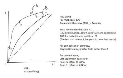
Receiver Operating Characteristic (ROC) Curve

We have mentioned binary diagnostic procedure. There is only a single set of sensitivity and specificity. However, tests may have values measured on numerical scales. For example, troponin level is a continuum to diagnose myocardial infarct. When the tests are measured on a continuum, sensitivity and specificity levels depend on where the cutoff is set between positive and negative results. ROC curve is a graphic plot to display the relationship in multi-level cuts.The ROC curve is created by plotting the true positive rate (TPR) against the false positive rate (FPR) at various threshold settings. The true-positive rate is also known as sensitivity. The false-positive rate is also known as (1-Specificity). There is a tradeoff between sensitivity & specificity. Sensitivity has an inverse relationship with specificity.When sensitivity raises, specificity drops.

Y-axis: true positive rate = TPR = sensitivity

X-axis: false positive rate = FPR = (1-specificity)

Slope = sensitivity / (1- specificity) = TPR/FPR = Positive Likelihood Ratio

Area under the curve (AUC) = Diagnostic Accuracy

Maximum value = 1

near 1 = excellent

0.8 - 0.9 = quite good

0.7 - 0.8 = moderately good

0.6 - 0.7 = marginally useful

0.5 or below = failed as a diagnostic test, just same as tossing a coin

The diagonal line: corresponds to a test that is positive or negative just by chance. This means that the AUC is 0.5, i.e.a useless test.Optimal point is defined as the point maximizing both sensitivity & specificity. The best point will be the left uppermost corner (most northwest point) that is closest to (0, 1) point.ROC curve can also tell the performance differences between 2 tests. Upper curve has larger AUC, and thus greater accuracy.

Cutoff points in screening and confirmation of disease

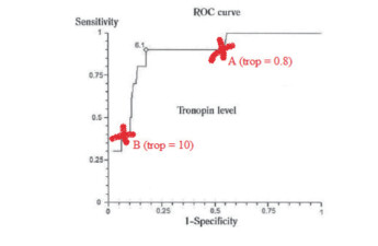
For a screening test, the cutoff point becomes more lenient. Sensitivity is increased and Specificity is decreased. False negative result is minimized.For a confirmatory test, the cutoff point becomes more stringent. Specificity is increased and Sensitivity is decreased. False positive result is reduced.For example, the diagram below represents the ROC curve for the diagnosis of AMI by troponin I (for illustrative purpose only):

When the cut-off criteria is more lenient (point A)

- Sensitivity is high,

- Specificity is low

- False negative rate is low

- SnNout to safely rule out when test is negative

When the cutoff criteria is more stringent (point B)

- Specificity is high,

- Sensitivity is low

- SpPin to safely rule in disease when test is positive

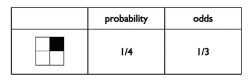
Relationship between probability and odds How to get odds from probability

Take Probability = p; Then odds = p / (1-p)

From above table, the probability of having shaded box is 1/4.

The probability of having unshaded boxes is 1- 1/4= 3/4

Odds of having shaded box is p /(1-p) = 1/3

Take another example. The probability of getting "1" after throwing a dice = 1/6.

Odds of getting "1" = (1/6) / (1-1/6) = 1/5

How to get probability from odds

By manipulating the equation further,

odds= p /(1-p)

odds (1-p) = p

odds - odds (p) = p

odds = p + odds (p)

odds= p (1+odds)

odds / (1+odds) = p

Hence, we get Probability (p)=odds /(1+ odds)

Applying the likelihood ratios to predict the posttest probability:

1.By calculation from pretest probability using the pretest & posttest odds:

Pretest probability

= The clinical likelihood before doing a test that the patient has the target disorder.

= Prevalence: proportion of people affected with a target disorder at a specified time.

Pretest odds

= The odds that the patient has the target disorder before the test is carried out

= Pretest probability / (1-pretest probability)

Posttest odds

= The odds that the patient has the target disorder after the test has been carried out

= Pretest odds x likelihood ratio

Posttest probability

= The proportion of individuals with that test result who have the target disorder, after the test is carried out and dependent on its result

= Posttest odds / (posttest odds + 1)

Further elaboration, say, Pre-test probability is 20%, PLR is 10

Step 1: Estimate or get pre-test probability from health data…supposing it is 20%

Step 2: Convert pre-test probability to pre-test odds

Pre-test odds = p / (1-p) =20/80 = 0.25

Step 3: Multiply pre-test odds by PLR to get post-test odds

Post-test odds= Pre-test odds x PLR = 0.25×10 =2.5

Step 4: Convert post-test odds back to post-test probability in percent

Post-test probability= Odds/ (1+odds) ×100 = 2.5/3.5×100~70%

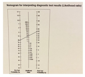
2.By Fagan's Nomogram (Likelihood Ratio Nomogram)

The nomogram can simplify the calculation of post-test probability. If we know the prevalence (pre-test probability) and the likelihood ratio of the test, we draw a straight line from the left (pre-test probability) to LR of the test; it anchors on the post-test probability on the right side.

Fagan's Nomogram: an example

Advantages of Likelihood Ratio:

- Not affected by Pretest Probability (Disease Prevalence)

- Enables you to go directly from Pretest Probability to Posttest Probability

- Can apply to Multiple Levels of test results and obtain Likelihood Ratio directly

Comments on the test characteristics:

(1) PPV and NPV change with different disease prevalence

(2) Sensitivity and Specificity become unstable when spectrum bias exists

(3) When a subject has positive results on diagnostic test, chance of having the disease is best estimated by post-test probability, rather than positive predictive value

Ⅴ、APPLICABILITY

1.5 Killer B's: Biology:SCRAP.Stands for Sex, Co-morbidity, Race, Age and Pathology

Bargain:a tradeoff between clinical benefits and harm/adverse effects

Barrier:availability/easy access of the test in your locality

Belief:patient's own beliefs/considerations

Burden:prevalence of the disease and financial concern

2.Threshold model:Test threshold & Treatment threshold

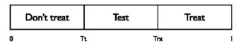
Medicine is an art. When facing diagnostic uncertainty, we may have our own judgment of probability of having a disease in our own patients. One can estimate the probability of the disease as a line that extends from 0 to 1.

The Testing threshold Tt is the point on the probability line at which no difference exists between the value of not treating the patient (Don't treat) and performing the test (Test).

Similarly, the Treatment threshold Trx is the point at which no difference exists between the value of performing the test (Test) and treating the patient without doing a test (Treat).

Tt and Trx vary among us because we have our own clinical judgment.If the probability of the disease is too low (< Tt), clinician would not perform the test to exclude the diagnosis or start treatment. If the probability is too high (>Trx), clinician would not perform the test to confirm the diagnosis and go straight to treat it directly. If the probability is in between Tt and Trx, clinician needs a test to confirm or exclude the diagnosis.

Factors affecting the treatment threshold:

(1) Disease itself

(2) Treatment cost

(3) Treatment adverse effect

Factors affecting the test threshold:

(1) Disease itself

(2) Test cost

(3) Test invasiveness

Diagnostic test will be useful if the result from pre-test probability to post-test probability crosses one of the threshold.

3.Individualizing the result by using local pre-test probability

The local prevalence of disease is our local pre-test probability.Value may be obtained by referring to our own local health figures.Using the patient's pre-test probability (based on clinical presentation or government data) and the Likelihood ratios based on the designated diagnostic test article, we anchor pre-test probability to estimate the patient-specific post-test probability using Fagan's Nomogram (Likelihood Ratio Nomogram).

End.