


2. School of Automation, Shenyang Aerospace University, Shenyang 110136, China;
3. School of Physics and Electromechnical Engineering, Zhoukou Normal University, Zhoukou 466001, China
2. 沈阳航空航天大学 自动化学院, 辽宁 沈阳 110136;
3. 周口师范大学 自动化学院, 河南 周口 466001
The selection and design of airfoil shapes is important work in aircraft design. Airfoils have a fundamental effect on the aerodynamic performance of aircraft. For today’s high-performance aircraft,directly selecting wings from the library of airfoils is no longer suitable. Instead,the initial airfoil must be optimized to become the specific wing that satisfies the performance requirements.
Most research on aerodynamic optimization relates to subsonic and transonic aircraft. However,with the increasing demand for civilian aircraft,low carbon and environmentally friendly electric aircraft are gradually being developed. The development cycle for their production needs to be shortened while their higher lift to drag ratio must be maintained. Aerodynamic optimization involves many aspects,one of them being parameterization for airfoil shape. There are several methods of parameterization,such as the Parametric Section Method (Parsec Method)[1],the Hicks-Henne shape function[2],B-spline curves[3],Mesh points[4],and the Class-Shape function Transformation (CST)[5]. The Hicks-Henne shape function and the Parsec Method are usually used in parameterization[6]. The former is common but cannot describe the airfoil’s trailing edge precisely. The latter is more common in research on supercritical airfoils.
The process of airfoil design is performed by iterations of numerical calculations and optimizations,so numerical calculation is an important section. Most numerical calculation is based on Computational Fluid Dynamics (CFD). Precise aerodynamic calculations require complex mesh modeling and thousands of iterations,and many researchers put a lot of effort into reducing the burden of numerical calculation,by using the multi-level algorithm by Kozie[7-8],for example. On the other hand,it is difficult for large-scale CFD calculation software such as Fluent to make seamless connections to Matlab,which demands excessive manual operations between numerical calculations and optimizations. This potentially increases the time cost in airfoil design. Professor Mark Drela of the Massachusetts Institute of Technology developed XFOIL software,which can improve the efficiency of numerical calculations within a certain range of accuracy[9]. In recent years,taking advantage of the speed made possible by XFOIL,more and more researchers have begun to use it in airfoil design[10-11]. However,due to the limited accuracy of XFOIL,it is more suitable for quickly finding the suboptimal solution,one which can be utilized as the initial airfoil for further design.
Genetic Algorithm (GA) is a common algorithm used in optimization by computer-aided design[12]. Ref.[13] studies the convergence behaviors of GA in aerodynamic optimization and points out that the optimization is affected not only by parameters of GA but also by numerical calculation. Besides GA,adjoint algorithm[14] and differential evolution algorithm[15] are also important methods. Most of research on aerodynamic optimization has focused on how to improve the accuracy of optimum solutions,but few of them have involved efficiency. Reaching the vicinity of the global optimum quickly and taking it as the initial value for optimization will save more time than searching for the optimum airfoil directly from the library.
To improve the efficiency of airfoil design,a real-coded genetic algorithm with variable resolution for rapid multi-objective optimization is studied in this work. The method will quickly find the suboptimal solution,which can be taken as the initial airfoil in the preliminary design stage. First,the defect in the Hicks-Henne shape function is improved. Then,real-coded chromosomes,crossover operators with variable resolution and dynamic penalty are designed in genetic algorithm for rapid optimization. Finally,a solution is proposed for multi-objective and multi-point optimization.
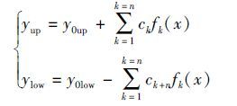
1 Airfoil geometry definition 1.1 ParameterizationA variety of methods have been developedto describe airfoil geometry,such as the series of NACA airfoils that have fixed analytical expressions[16]. In most cases,it is difficult or impossible to identify the specific geometry analytical expression of a general airfoil. Therefore,Hicks and Henne proposed a geometric representation of airfoils[17]. They used a set of smooth functions to perturb the standard geometry,and the main idea of this theory is the following:
|
(1) |
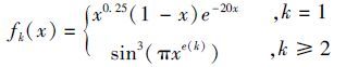
where fk(x) is called the shape function,and its expression is the following:
|
(2) |

|
(3) |
here,yup and ylow are the function of the upper and lower surfaces of the airfoil,respectively. y0up and y0low are the functions of the upper and lower surfaces on a standard airfoil,respectively. n is the number of shape function. ck is the coefficient of fk(x) and also the design variable. In Eq.(2),the first shape function f1(x) controls the range of airfoils in the leading edge,and others control the remaining parts together.
Studies have shown that almost all of the tails will overlap in practical application[18],and this causes the design space to be insufficient. Theoretically,“more than enough” design variables mean the shape functions are also “more than enough,” and the overlap will disappear. However,in fact,too many design variables will result in complicated parameterization and an increased workload in optimization.
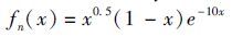
1.2 Improvement of Hicks-Henne shape functionIn the original research[17],Hicks and Henne referred to a kind of shape function in the trailing edge as in Eq.(4),but it requires the target and standard airfoils to be relatively similar.
|
(4) |
The derivative of Eq.(4) is the following:

|
(5) |
when x∈[0.7,1]. Eq.(4) and Eq.(5) are shown in Fig. 1. In the figure,the line with circles is the performance of original Hicks-Henne shape function on the trailing edge,and line with triangles represents its derivative.
Fig. 1 shows the value of the original Hicks-Henne shape function is close to zero on the trailing edge,and it means the function changes little there. The trend is also shown by its derivative. So the shape of the trailing edge remains almost unchanged.

|
| 图 1 原始Hicks-Henne型函数的后缘扰动函数及其导函数 Fig. 1 Original Hicks-Henne shape function and its derivative on the trailing edge |
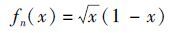
In aerodynamic design,the more precise the airfoil geometry is,the better. Therefore,the improved shape function on the trailing edge is as follows:
|
(6) |
The improved function and its derivative are shown in Fig. 2. In the figure,the line with circles is the performance of the improved Hicks-Henne shape function on the trailing edge,and the line with triangles is the performance of its derivative.

|
| 图 2 改进后的Hicks-Henne型函数的后缘扰动函数及其导函数 Fig. 2 Improved Hicks-Henne shape function and its derivative on the trailing edge |
Fig. 2 shows that the rake ratio of the improved function and its derivative is bigger than the original ones,which means the design space is expanded. Moreover,the improved function guarantees y(x)=0 at x=1.
2 Calculation of aerodynamic parameters 2.1 Numerical calculationWhen solving the flow around airfoil,the method based on the Euler equation or N-S equation coupled with the IBL equation requires a dense grid,so it will be very time consuming. In addition,airfoil design is necessarily a process of iterations and amendments. Time cost and accuracy are equally important,so XFOIL is engaged in the numerical calculation instead of large-scale software applications such as FLUENT and Ansys.
As previously noted,XFOIL was written by Professor Mark Drela at the Massachusetts Institute of Technology[19]. It is based on the non-viscous vortex panel method with linear strength. Through the distribution of source and sink on the surface and trailing edge of the airfoil,the effect of the viscous boundary layer on potential flow is simulated,and the viscous boundary layer is calculated by integral equation of the boundary layer. XFOIL is an important tool in low Reynolds numerical calculation,and its accuracy and reliability have been verified in many studies[20-21]. Moreover,according to Ref.[22],the paper calculates the aerodynamic performance of Eppler 387 and compares the results with the wind tunnel test. The comparative results show that the numerical data from XFOIL are close to the aerodynamic behavior of those in the real flow field.
XFOIL is commonly used to compute aerodynamic coefficients of airfoil sections.It is suitable for the calculation of low Reynolds numbers and will be questionable for highly separated and unsteady flow. The code operates with a viscous-inviscid interaction approach using “transpiration velocity”. When in subsonic,Karman-Tsien compressibility correction is also used. When in transonic or supersonic,the precision declines and cannot capture shock. The flow around a body is modelled with potential flow which is modified to take into account the viscous effects of the boundary layer. The transition point can be directly defined or the eN method can be used. The latter assumes that in the boundary layer,tracking waves are calculated for the stability diagram.
XFOIL maintains the boundary layer geometry information from each angle of attack analysis point and uses that information to initialize the computation at the next point. Consequently,by taking small steps in angel of attack,convergence will be reasonable. If higher angles of attack,the definition is quite different,XFOIL begins to show a totally different boundary layer characteristic: it predicts a laminar separation bubble which is a part of the modelling capability of the code[19]. In addition,oversized thickness or concave airfoil will cause the failure of calculation.
2.2 Hybrid calculation based on Matlab and XFOILAlthough XFOIL does not require mesh modeling,it still needs some parameters to be input manually in each iterative process,and this manual input is very cumbersome. Taking Matlab as the main platform of optimization and XFOIL as the external function for aerodynamic calculations,we designed an interface between Matlab and XFOIL.
Suppose the design Reynolds number is estimated to be about Re=6×10⁶ depending on the radial location,and the Mach number at the blade tip is set to M=0.5. Numerical computations go through each angle of attack between -5° and 15°.
| Instructions | Meanings |
| LOADAirfoil.dat | Load airfoil data |
| TEST | Test airfoil data |
| PANE | Set the number and position of the points |
| OPER | Set initial conditions for calculation |
| VISC 6×10⁶ | Set Reynolds |
| M 0.5 | Set Mach |
| ITER 150 | Set the number of iterations |
| PACC | Open the pole curve output |
| ASEQ -5 15 1 | Set the angle of attack sequence |
| Save.txt | Save calculation results |
All the aforementioned flow conditions are written as an input script.
The script is organized based on the following steps:
1) Input parameters. First input the parameters of the airfoil,which is a text file of coordinates. The coordinates are based on the initial settings,and they always change along with iterations. Each line of the text represents a coordinate point. From the top line to the bottom line,the coordinates sequentially represent the points from the trailing edge,continue counterclockwise around the leading edge,and finally return to the trailing edge.
2) Write script. The script is recognized by XFOIL code and named “Execution.vbs.” The main instructions of the script are listed in Table. 1. The line “Wscript.Stdout.WriteLine” should be added before each instruction. To ensure the instructions can be executed correctly,the line “Wscript.Sleep 1” should appear after each line of instructions.
3) Start script. Add “!Start.bat” in Matlab,and then the script will be imported to XFOIL and run. In Start.bat,“Cscript.exe//NoLogo Execution.vbs |xfoil.exe” should be written.
4) Output parameters. Store the results from XFOIL in the same directory for Matlab. The results may include the pressure coefficient,lift coefficient,drag coefficient,moment coefficient,etc. During the optimization process,the values of these aerodynamic parameters also change.
3 Improved genetic algorithm with variable resolutionMost design processes start with a standard airfoil from a library,and then a lot of time is spenton finding the special airfoil which satisfies the requirements. To improve the efficiency of optimization,the process can find the suboptimal airfoil first and then search for the optimal airfoil. Based on this idea,an improved genetic algorithm with two variable resolutions is proposed.
3.1 Real-coded technologyIn standard genetic algorithm,encoding is generally binary. Binary encoding is similar to the composition of biological chromosomes,so the algorithm can easily be explained by biological genetic theory,and genetic operations such as crossover and mutation are easier to be realized. However,in solving continuous optimization problems,there will be the following difficulties.
1) Binary encodings of two adjacent integers may be quite different,and this will reduce the efficiency of genetic operators.
2) The length of a gene is determined by the precision of the solution,and the length is difficult to change during the execution of the algorithm. If high precision is selected at the beginning,the gene length will be too long. In short,binary encoding lacks flexibility.
3) During the process of parameterization,encoding and decoding between binary and decimal is repeated many times,and this increases the amount of computation.
By using real code,all the genetic operations are carried out in the problem space directly. On the other hand,real code can overcome the above shortcomings and improve the performance of the optimization algorithm.
3.2 Crossover operators with variable resolutionCrossover operators play a central role in genetic algorithm,the role of determining the search capability. The principle of variable resolution is a two-stage optimization strategy aimed at the problem of lengthy searches caused by solution space that is multi-objective and large scale.
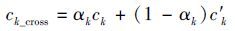
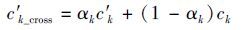
In a certain generation of the optimization process,suppose {ck} and {c′ k} are the parent individuals that are chosen as crossovers,k=1,2,…,n,and n is the number of shape functions. In the first stage of optimization,the algorithm searches in a relatively wide range,and it is easy to approach the optimal solution rapidly. According to Eqs.(7) and (8),crossover occurs between {ck} and {c′ k}
|
(7) |
|
(8) |
where k=1,2,…,n. {ck_cross} and {c′ k_cross} are the new individuals after crossover between {ck} a nd {c′ k} respectively. αk is a random number in [0, 1]. If ∀k,all the αk are equal,the crossover is overall cross.
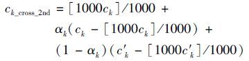
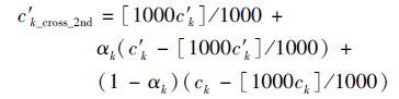
In the second stage of optimization,the algorithm searches in a relatively small range,and it is easy to find the optimal solution. The method reserves the highest bit and makes crossover between the remaining bits. For the general airfoils,the range of ck is (-0.007,0.007),so 0≤|ck|<0.01. Then,the crossover is shown by Eqs.(9) and (10) in the second stage of optimization.
|
(9) |
|
(10) |
where [ ] is the operation of reserving an integer.
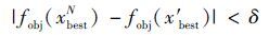
It is hard to determine when the transition from the first to second stage is complete. When the search slows down,the process is considered to be transferring from the first to the second stage of optimization. According to this characteristic,Eq.(11) is given as the switching point between the different stages.
|
(11) |
where x′ best is the best individual in all generations,and xNbest is the best individual of current generation N. fobj is the fitness function,and δ is the threshold. When the difference between the fitness functions is less than δ,convergence is considered to be slow,and the process is transferring from the first to the second stage of optimization.
The principle of variable resolution is also suitable for the mutation operator,and it can maintain the diversity of population in different degrees. In the first stage of optimization,ck is directly used in mutation,and the search is rapid and rough. In the second stage of optimization,one bit of ck is randomly selected to mutate,and the search is fine.
3.3 Dynamic penaltyIn standard genetic algorithm,encoding is generally binary. Binary encoding is similar to the composition of biological chromosomes,so the algorithm can easily be explained by biological genetic theory,and genetic operations such as crossover and mutation are easier to be realized. However,in solving continuous optimization problems,there will be the following difficulties.
Dynamic penalty is used together with variable resolution. In the first stage of optimization,discrete degrees of search points in the solution space are large,and the optimal solution may be lost. In the second stage of optimization,discrete degrees of search points are small,and there is little difference between solutions. This causes slow convergence.
To solve these problems,the original fitness function should be improved. In the first stage of optimization,the algorithm should collect as much global information as possible,so little penalty is imposed on the design points that violate the constraints. In the second stage of optimization,the algorithm should get sophisticated design results with high computational efficiency,so high penalties are imposed on the design points that violate the constraints.
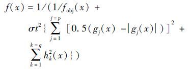
In order to adjust the penalty in proper time,the original fitness function is improved by a dynamic penalty function,and the new fitness function is the following:
|
(12) |
where fobj(x) and f(x) are the original and new fitness functions,respectively. gj(x) and hk(x) are the equality and inequality constraints,respectively. Here j=1,2,…,p,and k=1,2,…,q. t is the number of the current generation,and σ is a constant used to control the penalty.
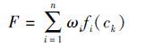
4 Solution of rapid optimization on airfoil shape 4.1 Multi-objective optimization and multi-point optimizationMulti-point and multi-objective optimization are different. In multi-objective optimization,the objective function consists of variables with different properties. For instance,the lift coefficient,drag coefficient,and moment coefficient can constitute an objective function. In multi-point optimization,the objective function consists of variables with the same property. It selects multiple design points of the same variable in a certain range. For instance,if the constraint requiring lift should reach a threshold when the angle of attack is in a certain range,the objective function will consist of lift in a different angle of attack. As in Eq.(13),both objective functions can be calculated by weighting the coefficient.
|
(13) |
where F is the objective function. ωi∈(0,1) is the weighting coefficient,and $\underset{i=1}{\overset{n}{\mathop{\Sigma }}}\,$ωi=1. ck is the coefficient of shape function and also the design variable. In multi-objective optimization,n is the number of variables,and fi is the function of the ith variable. In multi-point optimization,n is the number of design points,and fi is the function of the i th design point.
4.2 Integrated design methodThe process of airfoil design not only needs to satisfy a variety of constraints but also to reach multiple objectives. Being multi-constraint and multi-objective are the most important characteristics of the process. On the other hand,the problem of flow around is analyzed by numerical calculation,and the aerodynamic data is provided to the optimization algorithm. According to the above,the design process can be summarized as the following steps.

|
| 图 3 整体优化设计流程图 Fig. 3 Diagram of design and optimization |
1) Initial population is randomly generated in genetic algorithm,and each individual represents a set of design variables {ck}. It should be noted that the number of design variables in non-symmetrical airfoil are twice as much as in symmetrical airfoil.
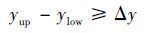
2) The airfoils described by individuals of each generation are tested by geometric constraints. If the airfoil does not satisfy the constraints,the individual will be punished. The larger the differences between individual and criteria,the greater the probability of elimination. Eq.(14) is the constraint of minimum thickness,and Eq.(15) is the constraint of wave wing.
|
(14) |
|
(15) |
In Eq.(14),Δy is minimum thickness. In Eq.(15),x′ i=xi+1-xi and x″ i=(xi+2-xi+1)-(xi+1-xi). The calculation of y′ i and y″ i is the same as x′ i and x″ i. xi is the coordinate on chord,and yi is the vertical coordinate of the upper or lower surfaces. k is the rake ratio. When the rake ratio of any two lines on the surface changes more than once,the airfoil is wave wing. Wave wing is an impractical airfoil and should be eliminated.
3) After a series of genetic operations,the next generation is generated,as are the new airfoil shapes. Then,the airfoil data is imported to XFOIL for numerical calculations.
4) When an individual can reach the desired target,or the number of iterations exceeds the maximum limit,the calculation is terminated.
5 Results 5.1 Simulation of improved Hicks-Henne shape functionMulti-point and multi-objective optimization are different. In multi-objective optimization,the objective function consists of variables with different properties. For instance,the lift coefficient,drag coefficient,and moment coefficient can constitute an objective function. In multi-point optimization,the objective function consists of variables with the same property. It selects multiple design points of the same variable in a certain range. For instance,if the constraint requiring lift should reach a threshold when the angle of attack is in a certain range,the objective function will consist of lift in a different angle of attack. As in Eq.(13),both objective functions can be calculated by weighting the coefficient.
Fig. 4 and Fig. 5 show the airfoil on the trailing edge described by the original Hicks-Henne shape function and the improved Hicks-Henne shape function with different ck,respectively. A comparison of Fig. 4 and Fig. 5 shows that the improved Hicks-Henne shape function can greatly change the airfoil on the trailing edge.

|
| 图 4 原始Hicks-Henne型函数的翼型后缘 Fig. 4 Airfoil described by original Hicks-Henne |

|
| 图 5 改进的Hicks-Henne型函数翼型后缘 Fig. 5 Airfoil described by improved Hicks-Henne |
5.2 Rapid design and optimization of airfoil
The number of shape functions in Eq.(1) is n=6. Because the airfoil is nonsymmetrical,there are 12 design variables. xk could be chosen uniformly distributed or user defined[23]. According to our early experiments,when k=1,2,3,4,5,6,xk is set to 0,0.2,0.4,0.6,0.8,and 1.0,correspondingly. The target of optimization is as follows:
1) When the lift coefficient is CL∈(0.9,1.3),the demand of the lift to drag ratio is CL/CD≥150.
2) When the angle of attack is α=0°,the demand of the pitch moment coefficient is Cm≥-0.11.
3) The maximum lift coefficient is not less than 1.75.
The constraints include the following:
1) The ranges of design variables are in Table 2.
| Design variables | Upper limit | Lower limit | Design variables | Upper limit | Lower limit |
| c1 | -0.006 | 0.006 | c7 | -0.006 | 0.006 |
| c2 | -0.004 | 0.006 | c8 | -0.006 | 0.004 |
| c3 | -0.004 | 0.007 | c9 | -0.007 | 0.004 |
| c4 | -0.004 | 0.007 | c10 | -0.007 | 0.004 |
| c5 | -0.005 | 0.005 | c11 | -0.005 | 0.005 |
| c6 | -0.005 | 0.005 | c12 | -0.005 | 0.005 |
2) The constraint of minimum-maximum thickness is 0.12 in Eq.(14).
3) The constraint of wave wing is Eq.(15).
The parameters of genetic algorithm are as follows. The scale of the initial population is 150,and the number of evolutions is 80. In the genetic operators,the probability of crossover and mutation is 0.9 and 0.02,respectively. The threshold of variable resolution in Eq.(11) is δ=50,and the constant of penalty in Eq.(12) is σ=0.5.
In the numerical calculation,the Reynolds number is 6×10⁶,the Mach number is 0.5,and the number of iterations is 150.
In the simulation,Ref.[24] is taken as a comparison to the method of this paper. Ref.[24] uses Elitist Nondominated Sorting Genetic Algorithm (NSGA-II) in the optimization of a wind turbine airfoil,and NSGA-II has an explicit diversity-preserving mechanism.
In comparison,the parameters of NSGA-II are the same as those in this paper.Fig. 6 shows the airfoil shapes before and after optimization. Fig. 7 presents the lift to drag ratios at different angles of attack. Fig. 8 gives the lift against lift to drag ratios. In these figures,solid lines represent the initial airfoil,dot-and-dash lines represent NSGA-II,and lines with stars represent the method presented in this study.

|
| 图 6 原始翼型与优化翼型对比 Fig. 6 Airfoil shapes before and after optimization |

|
| 图 7 升阻比随迎角变化曲线对比 Fig. 7 Lift to drag ratios at different angles of attack |

|
| 图 8 升阻比随升力系数变化曲线 Fig. 8 Lift against lift to drag ratios |
In Fig. 6,the maximum relative thickness of the original airfoil is at 28.5%c. Maximum camber is 2.6% at 48%c. After the optimization of NSGA-II,the maximum relative thickness is at 32.4%c. The maximum camber is 3.3% at 68%c. After the optimization presented in this study,the maximum relative thickness is at 34%c. The maximum camber is 4.1% at 75%c. In general,the positions of the maximum thickness and the maximum camber both move to the trailing edge after optimization. The offsets of this study are more obvious than those of NSGA-II. Moreover,the maximum camber increases after optimization,and the increment of this study is greater. These changes will improve the lift.
In Fig. 7,the lift to drag ratios at different angles of attack increase after optimization,and the phenomenon is more obvious in the method presented in this study. By using NSGA-II,the maximum lift to drag ratio increases 49%,and the stall angle of attack moves backwards as compared to that of the original airfoil. By using the method presented in this study,the maximum lift to drag ratio increases 59%. Although the stall angle of attack is ahead of that in NSGA-II,the stall characteristic is more moderate.
In Fig. 8,the lift against lift to drag ratios in this study are better than those of NSGA-II. The line of this paper shows when CL∈(0.9,1.3),CL/CD≥150,which satisfies the target of optimization,and the peak of CL/CD is 185. The line of NSGA-II shows when CL∈(0.9,1.3),CL/CD is close to 150.
NSGA-II was also employed for comparison with the method presented in this paper,and the time consumed as a result is shown in Table 3. Two major factors were investigated: 1) the CPU time for the optimal procedure and 2) the solution of the optimization. The calculations were conducted with a computer with an Intel 4.0 GHz core i74790K CPU and 8 GB of RAM. In the previous experiment,the Reynolds number was 6×10⁶,the Mach number was 0.5,and the number of iterations was 150.
As Table 3 shows,XFOIL is faster than FLUENT in the numerical calculation,the CPU time for each is 10~25s and 1~2min,respectively. After 150 iterations,the improved GA with variable resolution presented in this study reaches the maximum lift to drag ratios at 185 within 4h. In contrast,NSGA-II reaches the maximum lift to drag ratios at 146 within 10h. Table. 3 shows that the improved GA with variable resolution presented in this study is more efficient in the speed of calculation and gets better results.
| Operation | Result | CPU time | |
| XFOIL | ~ | 30~50s/iteration | |
| FLUENT | ~ | 3~4min/iteration | |
| Improved GA | 185 maximum CL/CD | within 4 hours | |
| NSGA-II | 146 maximum CL/CD | within 10 hours |
It should be noted that the method presented in this study and NSGA-II are the same kind of optimization method. In the case of infinite iteration,both of them will find the same optimum solution,theoretically.It should be noticed that all the results above are obtained with insufficient iteration and the performance of two methods will be close to each other as the increase of iterations. Furthermore,when the simulation time exceeds 14h,the results of NSGA-II will be better.
The method presented in this study pays more attention to the efficiency of the search,so it will approach the optimum solution more rapidly in the early stage.Moreover,the numerical calculation of XFOIL will result in less time cost than if some large-scale software application is used. Overall,the method presented in this study will be more efficient. Therefore,the method is particularly suitable in the early stage of design,such as for the selection of initial airfoil shape or the rapid definition of a new shape,where the development cycle needs to be shortened.
6 ConclusionAn improved genetic algorithm with variable resolution for the rapid design of airfoils has been studied. Comparison and analysis have yielded the following useful conclusions.
1) The improved Hicks-Henne shape function has better performance on the trailing edge than does the original. Because the trailing edge is important to the aerodynamic behavior,the improved Hick-Henne shape function is more suitable for the parameterization of the airfoil shape.
2) The improved genetic algorithm is more efficient because of the design of real-coded technology,searches with variable resolutions,and dynamic penalties. Combined with XFOIL in numerical calculation,the integrated solution can shorten the development cycle,so it will be valuable in engineering applications.
3) In the early stages of design,the method can quickly approach the optimum solution. This makes it suitable for the selection of the initial airfoil shape or the rapid definition of a new shape. Airfoils designed by this method may not meet some stringent aerodynamic requirements,so they will need further optimization before they can be used.
| [1] | Vecchia P D, Daniele E, Amato E D. An airfoil shape optimization technique coupling PARSE parameterization and evolutionary algorithm[J]. Aerospace Science and Technology, 2014, 32(1):103–110. DOI:10.1016/j.ast.2013.11.006 |
| [2] | Duan Y H, Cai J S, Li Y Z. Gappy proper orthogonal decomposition-based two-step optimization for airfoil design[J]. AIAA Journal, 2012, 50(1):968–971. |
| [3] | Sommer L, Bestle D. Curvature driven two-dimensional multi-objective optimization of compressor blade sections[J]. Aerospace Science and Technology, 2011, 15(1):334–342. |
| [4] | Boris A. 2D structured grid generation method producing a mesh with prescribed properties near boundary[J]. Engineering with Computers, 2012, 28(1):409–418. |
| [5] | Liao Y P, Liu L, Long T. Multi-objective aerodynamic and stealthy performance optimization for airfoil using kriging surrogate model[C]//2011 IEEE 3rd International Conference on Communication Software and Networks. NJ, United States: IEEE Press, 2011: 569-574. |
| [6] | Jeong S, Murayama M, Yamamoto K. Efficient optimization design method using kriging model[C]//AIAA Aerospace Sciences Meeting and Exhibit. United States. United States: AIAA Press, 2004: 1-10. |
| [7] | Koziel S, Leifsson L. Multi-level CFD-based airfoil shape optimization with automated low-fidelity model selection[J]. Procedia Computer Science, 2013, 18:889–898. DOI:10.1016/j.procs.2013.05.254 |
| [8] | Koziel S, Leifsson L. Automated low-fidelity model selection for CFD-based aerodynamic shape optimization[C]//10th AIAA Multidisciplinary Design Optimization Specialist Conference. United States: AIAA Press, 2014: 1-8. |
| [9] | Drela M. XFOIL subsonic airfoil development system[EB/OL]. http://web.mit.edu/drela/Public/web/xfoil/. 2014-10-17/2015-01-03. |
| [10] | James G, Zhang X, Phillip J, et al. Effects of real airfoil geometry on leading edge gust interaction noise[R]. AIAA 2013-2203, 2013. |
| [11] | Zhu W, Shen W Z, Srensen J N. Integrated airfoil and blade design method for large wind turbines[J]. Renewable Energy, 2014, 70:172–183. DOI:10.1016/j.renene.2014.02.057 |
| [12] | Yoshida E, Murata S, Kamimura A, et al. Evolutionary motion synthesis for a modular robot using genetic algorithm[J]. International Journal of Automation Technology, 2003, 15(2):227–237. |
| [13] | Cinella P, Congedo P M. Convergence behaviours of genetic algorithms for aerodynamic optimisation problems[J]. International Journal of Engineering Systems Modelling and Simulation, 2013, 5(4):197–216. DOI:10.1504/IJESMS.2013.056782 |
| [14] | Luo J Q, Xiong J T, Liu F. Aerodynamic design optimization by using a continuous adjoint method[J]. Science China: Physics, Mechanics and Astronomy, 2014, 57(7):1363–1375. DOI:10.1007/s11433-014-5479-0 |
| [15] | Derksen R W. BEZIER-parsec: an optimized airfoil parameterization for design[J]. Advances in Engineering Software, 2010, 41(7-8):923–930. DOI:10.1016/j.advengsoft.2010.05.002 |
| [16] | Senthil K S, Sankar G M, Kamalakannan K, et al. Design and computational analysis of NACA 846A110 and NACA 837A110 airfoils[C]//Proceedings of the 37th National and 4th International Conference on Fluid Mechanics and Fluid Power. NJ, United States: IEEE Press, 2010: 1-11. |
| [17] | Hicks R M, Henne P A. Wing design by numerical optimization[J]. Journal of Aircraft, 1978, 15(7):408–412. |
| [18] | 陈 学孔, 郭 正, 易 凡, et al. 低雷诺数翼型的气动外形优化设计[J]. 空气动力学学报, 2014, 32(3):300–307. |
| [19] | Drela M. XFOIL: an analysis and design system for low Reynolds number airfoils, low Reynolds number aerodynamics[J]. Lecture Notes in Engineering, 1989, 54:1–12. DOI:10.1007/978-3-642-84010-4 |
| [20] | Levin O, Shyy W. Optimization of a flexible low Reynolds number airfoil[R]. AIAA 2001-0125, 2001. |
| [21] | Antunes A P, Azevedo L F, Silva R G. A framework for aerodynamic optimization based on genetic algorithms[R]. AIAA 2009-1094, 2009. |
| [22] | Selig M S, Deters R W, Williamson G A. Wind tunnel testing airfoils at low Reynolds numbers[R]. AIAA 2011-875, 2011. |
| [23] | Wang Z, Yu S J, Liu T G. Effect of shape parameterization on aerodynamic shape optimization with SPSA algorithm[C]//Parallel Computational Fluid Dynamics 25th International Conference. Germany:[WX)][WX(4.5mm,75.5mm] Springer Verlag, 2014: 393-402. |
| [24] | Huque Z, Zemmouri G, Harby D, et al. Optimization of wind turbine airfoil using nondominated sorting genetic algorithm and pareto optimal front[J]. International Journal of Chemical Engineering, 2012(2012):1–9. |