


2. 空气动力学国家重点实验室, 四川 绵阳 621000;
3. 国家CFD实验室, 北京 100191
2. State Key Laboratory of Aerodynamics, Mianyang Sichuan 621000, China;
3. National Laboratory of Computational Fluid Dynamics, Beijing 100191, China
0 Introduction
In 1972, under the suggestion of Professor Hsue-Shen Tsien, Zhang H X turned his research interests of analytical solutions for hypersonic flows over blunt bodies[1]into the new field of Computational Fluid Dynamics.After that, he began to study the numerical method for compressible flow, such as some mixed explicit-implicit method for supersonic and hypersonic separated flow.In September 1978, the institute of measurement and computation was setup in China Aerodynamic Research and Development Center (CARDC) under the suggestion of Professor Hsue-Shen Tsien.A major part of the researchers in this institute begun their studies on CFD.In 1983, Computational Aerodynamics Institute (CAI) was set up in CARDC.In 1984, Zhang H X[2]found the relationship between the coefficients of modified equation and the numerical oscillation around shock wave. And then a numerical scheme was proposed to compute the supersonic flow without oscillation. This is the prototype of the NND scheme, which has been widely applied in the simulations of engineering problems and the study of numerous mechanisms. In this period, many researchers in China had become interested in CFD and began to study CFD, such as Zhuang F G in CARDC, Shen M Y in Tsinghua University, Dun Huang in Beijing University, Zhu Ziqiang in Beijing University of Aeronautics and Astronautics, Zhang Zhongyin in Northwestern Polytechnic University, Yang Zhasheng in Nanjing University of Aeronautics and Astronautics, Zhuang Lixian in University of Science and Technology of China, Wang Chengrao in National University of Defense Technology, Bian Yingui, Fu D X and Gao Zhi in Institute of Mechanics, Chinese Academy of Sciences and Wang Yiyun in China Academy of Aerospace Technology. Since then, CFD undertook fast development in China.
From July 2 to July 7 in 1982, the first national conference on computational fluid dynamics of China (NCCFD) was held in Chengdu, China. From then on, it was held biannually. Because of the development and contribution of CFD in China, two important streams of conference in CFD-International Conference on Numerical Methods in Fluid Dynamics, ICNMFD (since 1969) and International Symposium on Computational Fluid Dynamics, ISCFD (since 1985) had been successfully hold in China in 1986 and in 1997 respectively. From July 14 to 18, 2014, the eighth international conference on computational fluid dynamics (ICCFD), a merger of ICNMFD and ISCFD, was held successfully in Chengdu, China. It is interesting coincidence that this is the first time for China to host ICCFD and the city of Chengdu hosed the first NCCFD twenty two years early. China also held Asian Conference on CFD (ACFD) several times (Mianyang in 2000, Taiwan in 2005, Hongkong in 2010, Nanjing in 2012). Besides these conferences, there were many workshops and seminars on CFD in China, such as the most influential seminar held monthly in Beijing, the Sino-Japan workshop on CFD, the workshop on CFD cross the strait, and so on.
With the development of CFD, Zhuang F G and Zhang H X [3] noticed both the advantage and disadvantage of CFD technical. They pointed out that the greatest advantage of CFD is to obtain the detailed data of flow field and the impressive flow structures, while the serious disadvantage is the data ocean produced by CFD. Entering CFD era, more and more researchers strongly rely on CFD code, data and figures, ignore analysis on flow mechanisms. So Zhang H X advocated that CFD community should emphasize the integrated study of CFD and physical analysis. He has been focusing on the coupling study on CFD and physical analysis since he entered this field. From April 10 to 17 in 1983, the first national conference on flow separation and control (NCFSC) was held in Emei mountain, where is not far from Chengdu. This conference has been held biannually since then. The main purpose of NCFSC is to study the flow mechanism, in which CFD plays a very important role.
Zhang H X spent all his energy on the study of CFD and physical analysis. He has been the chairman of both NCCFD and NCFSC for more than thirty years. Based on the idea of integrated study of CFD and physical analysis, he proposed the principles to design numerical schemes, a concept of M5A for the area of CFD, NND scheme and a theory of steady and unsteady flow separation, which are considered as the landmarks or milestones of CFD and fluid mechanics in China. In this paper, the authors will give a brief review on these works.
1 Concept of M5A and Principles to Design Numerical Schemes 1.1 Concept of M5 AIn Ref.[3], Prof. Zhuang F G and Zhang H X classified the area of CFD into six branches, containing five “M”s and one “A”, which is marked by M5A. The five “M”s represent method, mesh, machine, mapping and mechanism respectively, while “A” means applications.
“Method” is the key issue and the most active branch in CFD. There are a lot of numerical methods such as finite difference methods, finite volume methods, finite element methods and spectral methods. “Mesh” is the foundation of CFD. It contains structured, unstructured and hybrid grids and moving mesh. “Machine” means the computers and supercomputers, which are the hardware resources of CFD. In recent years, computer science has achieved its fast development in China. The ‘Tianhe-II’ Supercomputer became the fastest machine in the world since 2013. Therefore, how to reach the full HPC potential of this supercomputer is an important issue for CFD. “Mapping” represents the visualization of numerical results, which is also a very important field to analyze the big data. “Mechanism” is the soul of CFD. With the powerful tool of CFD, we can obtain the solutions for Euler or Navier-Stokes equations, which are the governing equations of fluid motion. Based on this solution and coupled with physical analysis, we can reveal the detail mechanism of fluid mechanics, which forms the contribution to the development of fluid mechanics. Without the mechanism, CFD will lost its soul and go to an extreme direction to produce data ocean and pictures.
“Application” is the target of the CFD. The goal to construct the numerical method, to develop the software, is to promote applications in industry. Now CFD has become a more and more important tool for engineering design and optimization, especially in aeronautics and aerospace. This is the destination to develop science and technology. Fig. 1 shows the concept of M5A and relationship among the five “M”s and the “A”.
 |
| Fig. 1 Concept of M5A. |
Numerical scheme is the most important branch in CFD. Based on the analysis of the evolution of numerical error for the model equation and its modified equation, Zhang H X proposed four principles to design a rational numerical scheme. They are the criterion of dissipation controlling, the criterion of dispersion controlling, the criterion of capturing shock waves and the criterion of frequency spectrum controlling.
The first principle is the criterion of dissipation controlling. It requires that the combination of the coefficients of the dissipation terms is less than zero, which indicates that the coefficient of the leading dissipation term is less than zero. This is a necessary condition for the stability of the numerical scheme.
The second principle is the criterion of the dispersion controlling. It requires that the combination of the coefficients of the dispersion terms is less than zero on the left side of the shock wave, while larger than zero on the right side of the shock wave. It indicates that the coefficient of the leading dispersion term is less than zero on the left of the shock wave, and larger than zero on the right of the shock wave. This condition can suppress the spurious oscillation in the discontinuous region.
The third principle is the criterion of the frequency spectrum controlling. This means that the difference between the modified wave number and the exact wave number should approach to minimum. This is the key principle to design a high order numerical scheme to simulate multi-scale flow problems.
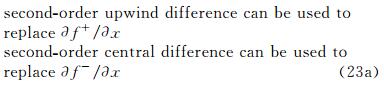
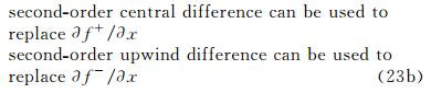
The fourth principle is the criterion of capturing the shock wave. In the numerical simulation of the flow structures with shock waves, the scheme is expected to capture the shock wave without any oscillation, and the Rankine-Hugoniot relationship should be satisfied. For second order numerical scheme, the third coefficient of the modified equation should be larger than zero on the left of the shock wave, and less than zero on the right of shock wave simultaneously. And the fourth coefficient will be negative. We refer to Ref.[4] for details.
2 Numerical Schemes 2.1 NND Scheme 2.1.1 Relationship Between Coefficient of Modified Equation and Spurious Oscillation around Shock [2]In 1984, Zhang H X [2] studied the evolution of numerical error for Navier-Stokes equation. He found the relationship between the coefficients of the modified equation and the spurious oscillation around the shock waves. Then, He proposed a numerical scheme through controlling the oscillation around shock wave, which is the prototype of NND scheme. Here, we give a brief review of this scheme.
The problem of one-dimensional shock wave is studied as an example using a time-dependent method. The model equation and boundary con-ditions are
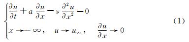
where
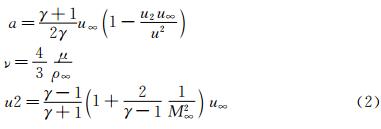
ρ, u, and μ are the fluid density, velocity and the viscous coefficient respectively. The variable t represents the time and x a coordinate (Fig. 2). Free-stream conditions are denoted with the subscript “∞”. M∞ is the free-stream Mach number and γ is the ratio of the specific heat. If the flow is steady and the viscous coefficient is constant, Eq. (1) represents the exact Navier-Stokes equations governing a normal shock wave.
 |
| Fig. 2 One dimensional shock wave. |
If a finite difference method is applied to solving Eq. (1), the modified differential equation after discretization can be rewritten as
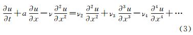
where the right-hand side represents the truncation error for the difference method. For a second-order difference method, ν2=0.
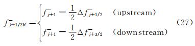
Now, we study the effects of coefficients ν2, ν3, … in Eq. (3) on the numerical solution. In fact, if the flow is steady, Eq. (3) can be integrated for one time to obtain
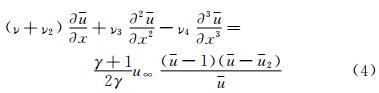
where
Here, u=1 is the nondimensional velocity in the upstream region of the inviscid shock, and u= u2 is the nondimensional velocity in the downstream region.
We assume that the numerical oscillations induced by the truncation error of the difference method are small. Then, in the upstream region of the shock,

and in the downstream region of the shock,

where u′<<1 in the upstream and u′<<u2 in the downstream. Substituting (5a) and (5b) into Eq. (4) and neglecting the high-order small quantity, we obtain
where,
Equation (6) is linear and its solution can be determined by following characteristic equations


There are two typical solutions under two following conditions.
Case 1 . ν2=0, ν3<0 and ν4 is very small. For inviscid flow (ν=0) or the flow at high Reynolds number (ν is very small), the solution of Eq. (6) is
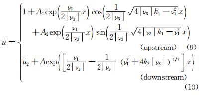
It is very clear that the spurious oscillations occur in the upstream region of the shock, but not in the downstream region.
Case 2 . ν2=0, ν3>0 and ν4 is very small. In a similar way, it can be proved that the spurious oscillations occur in the downstream region of the shock, but not in the upstream region.
These two cases correspond to the flow patterns using the second order difference scheme. Through the preceding study for one-dimensional Navier-Stokes equations, it is found that the spurious oscillations occurring near the shock with the second-order finite difference schemes are related to the dispersion term in the corresponding modified differential schemes. If we can keep ν3>0 in the upstream region of the shock and ν3<0 in the downstream, we may have a smooth shock transition, i.e., the undesirable oscillations can be totally suppressed (Fig. 2).
2.1.2 Physical Entropy and Numerical SimulationThe preceding conclusion can be verified by following physical discussion from the second law of thermodynamics. In fact, the one-dimensional Navier-Stokes equations modified by the addition of dispersion terms with coefficient ν3 are as follows:
Where p represents the pressure, H represents the total enthalpy, and the Prandtl number is assumed to be 3/4. From Eq. (11), we can obtain an equation of entropy s for the heat-isolated system
Here, Ds/Dt is the substantial derivative of entropy. For a true physical shock, we have, in the upstream of the shock,
Hence,
And in the downstream of the shock,
Hence,
For inviscid flow or flow with high Reynolds numbers, we may neglect the viscous contribution to the entropy. Therefore, we may observe that if ν3>0 in the whole shock region, the increasing entropy condition is met in upstream region but not satisfied in the downstream region. And this is associated with the appearance of spurious downstream oscillations. On the other hand, if ν3<0 in the whole region, the increasing entropy condition is not met in the upstream, and spurious oscillations occurs. Now, it is obvious that if we can keep ν3>0 upstream and ν3<0 downstream, we may have a smooth shock transition (Fig. 1).
To test the effectiveness of previous conclusion, we calculated one-dimensional flow with Eq. (11). Numerical results [5, 6] verified the preceding conclusion.
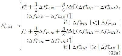
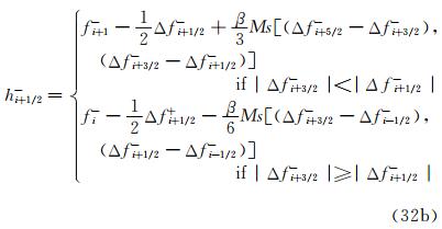
2.1.3 NND Schemes [5, 6, 7]Based on above considerations, Zhang H X proposed a second order non-oscillatory and non-free parameter dissipation (NND) difference scheme. We start with a one-dimensional scalar equation
Here, f=au and a=∂f/∂u, a is the characteristic speed, and we may write

where

Define

We have

Equation (1) may be rewritten as
In the upstream region of a shock:
In the downstream region of a shock:
Then we have made the proper choice of the sign of the coefficient of the third derivative in the modified differential equation, i.e., ν3 keeps positive in the upstream of a shock and negative in the downstream of a shock. And this will provide us with a sharp transition without spurious oscillations, both upstream and downstream of shocks. At the same time, we notice that the coefficient of fourth-order dissipative derivative is negative in the entire region, which can help to suppress odd-even decoupling in smooth regions of physical flows.
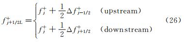
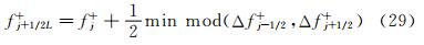
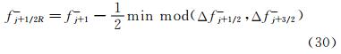
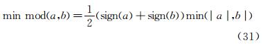
Now we have the semi-discretized difference form of Eq. (17) as follows:
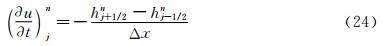
where,

and

2.1.4 Extension and Applications of NND Scheme
Since the birth of NND scheme, it has been studied and applied extensively in Chinese CFD community. It was extended to several versions ranging from NND-1 to NND-5 [6, 7]. Moreover, the finite difference version of NND scheme was extended to finite volume version [8] on unstructured and structured/unstructured hybrid grids. As an example, we just list a third order essentially non-parameter non-oscillation (ENN) scheme [9], which is an extension of NND scheme by careful designing of the limiters as follow.
There are many applications of NND schemes on flow mechanisms and computation of aerodynamics for engineering problems [8, 9, 10, 11, 12, 13, 14]. Fig. 3 contains the contours of a supersonic flow in a nozzle, which are obtained by several different versions of NND scheme. For comparison, we also provide the experiment picture. We can observe that the complex flow structure is captured clearly, and as the accuracy order increasing, the complex flow structure becomes clearer. Fig. 4 contains the time evolution of flow structure of a normal shock wave passing through a wedge in a tube. The numerical scheme is a fourth order weighted DRP scheme [13]. The flow structure is captured very clearly.
 |
| Fig. 3 A supersonic flow in a nozzle at t=1.5 ms. |
 |
| Fig. 4 Density contours of shock wave move around a wedge in tube (Ms=8.293) by a 4th-order HWDRP4. |
To compute the aerodynamics of engineering problems with complex configurations, a series of in-house software were developed based on the NND scheme in CARDC, such as the CFD platform for supersonic flow on structured grids-Chant, the CFD platform on unstructured and hybrid grids-HyperFLOW. These CFD codes were extensively applied to the engineering problems with complex configurations. Meanwhile, Zhang’s group had developed their grid generation techniques for unstructured and hybrid grids, and dynamic hybrid grids. As an example, we show the numerical simulation for the problem of a wing-pylon-store separation [14]. The unsteady solver is coupled with the six degree of freedom (6DOF) integration. The moving grids have been shown in Fig. 5. Fig. 6 shows the pressure contours during the store separation. In Fig. 7, the kinetic and aerodynamic parameters during separation are shown, and compared with experi-mental data [15] (marks in the figure). Note that the present results agree very well with the published results. In this case, the total number of cells is about 240M and a 32-processes parallel computing was adopted also.
 |
| Fig. 5 Dynamic grids during the store separation. |
 |
| Fig. 6 Pressure contours during store separation. |
 |
| Fig. 7 Kinetic and aerodynamic parameters during separation. |
Based on the principle of the suppression of the numerical oscillations, Shen M Y [16] proposed a class of generalized compact scheme for the model equation (1). It is
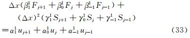
Where, Fj and Sj are approximations for  and
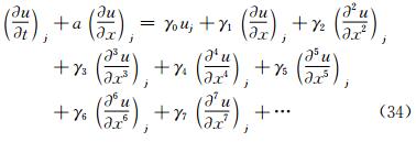
and  respectively. αmn, βmn and γmn are coefficients. After Taylor series expansion and successive differentiations for Fj and Sj, and substituting them into the model equation (1), it is easy for one to obtain the modified equation:
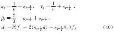
For fifth order accurate compact scheme, the coefficients are
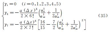
where αa1=α11+α-11 and αm1=α11-α-11 . The modified equation for the fifth order accurate compact scheme can be rewritten as
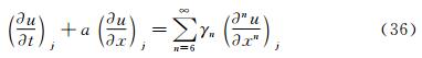
According to the principles about the construction of high-order accurate schemes proposed by Zhang H X shown in the previous section, the principle of stability is γ6>0 in the whole computational domain. The principle about suppression of the oscillations is
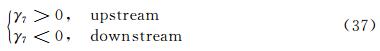
Following these conditions, one can obtain
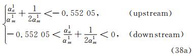
For the case of a>0, and
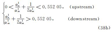
For the case a<0. From these conditions, one can obtain the coefficients αmn, βmn and γmn in Equation (33). We refer to the paper Ref.[5] for detail. Based on this scheme, Zhang et al. [17] proposed a space-time conservation schemes for three dimensional Euler equations.
2.2.2 A Compact Scheme with Group Velocity ControlFu D X and Ma Y W [18, 19] heuristically analyzed relationship between the oscillation around shock wave and group velocity of wavepackets of numerical scheme. They found that the oscillations in the numerical solutions are produced behind the shock wave if the group velocity of wavepackets with moderate and high wave numbers in the numerical solution is slower than the group velocity of the exact solution. The oscillations are produced in front of the shock if the group velocity of the wave packets with moderate and high wave numbers is faster than the group velocity of the exact solution. To suppress the oscillation, the method of diffusion analogy was used to control the group velocity of wavepackets so that the Fourier components in the numerical solutions have a faster group velocity of wavepackets behind the shock and a slower group velocity in front of the shock.
The compact scheme proposed by Fu and Ma has the following form

Where,
And σ is a parameter to control the group velocity of the numerical scheme, which is defined as
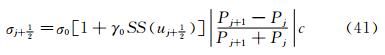
With 1≤σ0≤2 and 0.8≤γ0≤1. SS(u) is shock structure function, which is defined by SS(u)=sign . We refer to papers Refs.[18, 19] for details.
As the fast development of supercomputer, direct numerical simulation (DNS) has become a very powerful tool to study the mechanisms of multi-scale flows, such as turbulence and aeroacoustics. The simulations for these multi-scale problems need high order and high resolution numerical methods. To achieve this goal, Zhang’s group developed a series of high order, high resolution shock capturing schemes, including the weighted nonlinear compact schemes (WCNS) [20, 21, 22], a class of central compact scheme with spectral-like resolution (CCSSR) [23, 24, 25], improvement the convergence toward the steady state solution for weighted schemes [26, 27], WENN scheme and a class of hybrid schemes of discontinuous Galerkin and finite volume method (DG/FV) [28, 29, 30, 31]. Some of these high order numerical schemes have been applied to solve engineering problems with complex confi-gurations. Almost all of these schemes have been applied to study the mechanism of complex flow [32, 33, 34, 35, 36, 37, 38, 39, 40, 41, 42]. For example, Li and Fu [36, 37, 38, 39, 40, 41, 42] performed a class of DNS including isotropic (decaying) turbulence [36], turbulent mixing-layers [37], turbulent boundary layers [38, 39, 40, 41] and shock/boundary-layer interaction [42]. The mechanism, modeling and controlling techniques of compressible turbulence are studied based on the DNS data, which show that DNS is a powerful tool to study compressible turbulence. Fig. 8 shows the distribution of skin fraction coefficient on the surface of a cone from DNS data in Ref.[41], and it shows that transition line on the cone surface shows a non-monotonic curve. Fig. 9 shows the instantaneous temperature in a DNS study of compression ramp [42], which shows the complex patterns for a shock-turbulent boundary layer interaction flow. We refer to Ref.[4] for details.


To correctly compute the flow field described by Euler equations or Navier-Stokes equations, Zhang H X [43] proposed a criterion for grid size. The non-dimensional form of gas dynamics equations can be written as
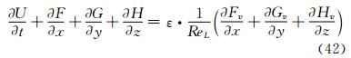
where x, y, z are the coordinates in the streamwise direction, circumferential and normal directions of the body surface, ReL is the Reynolds number. If ε=0, it is Euler equations. If ε=1, it is Navier-Stokes equations. If an m-th order difference scheme is adopted to simulate Equation (42), the semi-discretized modified differential equations corresponding to the difference equations are
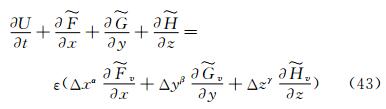
where α, β, γ are determined by following relations
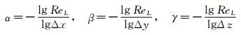
or
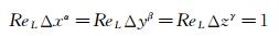
and
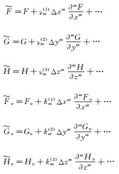
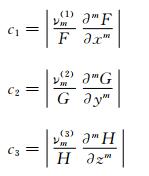
Δx, Δy and Δz represent the grid interval. νm(1), νm(2), …, km(3) are the coefficients of the m-th order truncation error terms.
In order to calculate correctly the flow fields described by Euler equations, the computational grids must satisfy the following requirement:

where
Now we discuss the computational grids for Navier-Stokes equations. In that case, Equation (43) can be further written as:
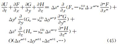
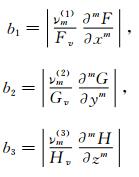
From Equations (45), together with conditions (44), the computational grids for Navier-Stokes equations should be chosen as follows:

where
Generally,  ,
,  and
and  are not very small, so we have to ask:
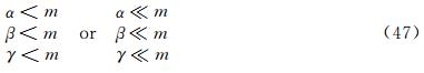
The conditions (46) and (47) mean that only if α, β and γ are all less or far less than m (the accuracy of the difference scheme used), the contribution of viscous terms are correctly calculated. In many references which adopt the second order scheme to solve Navier-Stokes equations (m=2), the grid interval do not meet the above requirement (46) or (47). Only in the direction z, γ<m is valid because the grid clustering technique is applied close to the body surface. In this case, it seems to solve the fully Navier-Stokes equations, but in fact it is just equivalent to solving viscous thin-layer approxi-mation equations.
According to the above discussion, the grid interval and the number should be designed in the computation according to above relations for every grid system. In recent years, we have developed the hybrid grid system based on the above requirements, which consists of structured, unstructured and rectangular grids. This system fits to the computation of complex flow field and can save CPU time.
4 Physical AnalysisFrom 60s to 80s of last century, there was a long-standing dispute regarding whether the separation line is an envelope of the limiting streamlines or the skin friction lines, or if itself is also a limiting streamline [44]. With the development of CFD, it was the best time to study this problem in terms of the physical analysis and numerical simulation. Moreover, in the numerical simulation and experimental tests, the flow structure is often examined through studying the surface flow on the body and cross-flows on the cross sections perpendicular to body axis. Hence, the topological rules of the surface flow and cross-flow are very important for analyzing the flow structure and mechanism.
4.1 Criteria of Flow SeparationIn Ref.[45] and [46], Zhang studied the criteria and flow pattern of steady separation described by Navier-Stokes equation and boundary layer equation respectively. To study the separation of three-dimensional steady flow on a fixed wall, we introduce two definitions: 1) Separation line is the intersection of wall and separation surface leaving the wall; 2) The solid wall can be regarded as a limit stream surface that attaches to the wall. Separation surface and wall z→0 are two different flow surfaces. Fig. 10 is a schematic diagram of the flow pattern near a separation line. Based on these definitions, Zhang H X proposed separation criteria.
 |
| Fig. 10 Schematic diagram of flow separation and coordinate system. |
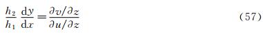
Suppose x, y and z are three axes of an orthogonal coordinate system. x and y are on the wall. z points toward the outward normal direction of wall. h1=h1(x, y, z), h2=h2(x, y, z) and h3=h3(x, y, z) are Lame coefficients in x, y and z directions respectively. Supposing the separation surface be z=f(x, y), the equation to describe the separation surface is:

After considering the geometrical relationship of separation pattern, we can obtain the separating angle between the wall normal direction and the normal direction of separation surface, which is
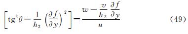
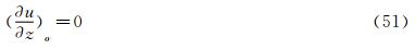
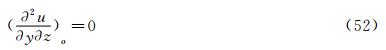
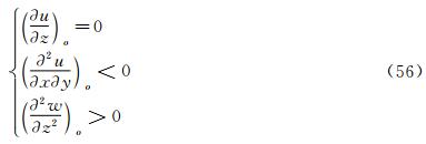
Supposing the separation line be y axis, the subscript “o” shows any point on the body surface. Because the flow described by Navier-Stokes equation has no Goldstein singularity at the separating line, Taylor series expansion can be used to the velocity components (u, v, w). They are
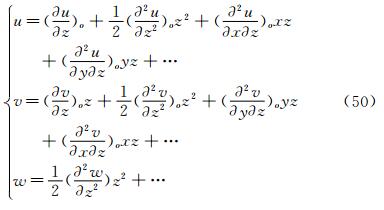
Where the boundary conditions uo=vo=wo=0 and  =0 from continuous equation are used. Using (49) and (50), we can obtain the following relations on the separation line.
Now, we consider the motion of flow in the near region of separating line. The equation is
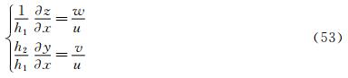
The first equation represents the characteristic of flow in the cross section perpendicular to the separating line. The second equation represents the flow characteristic in the section parallel to the plane of xoy. As z→0, it represents the limiting streamline on the wall. Substituting (50) into (53) on the separation line and neglecting high order term, we can obtain
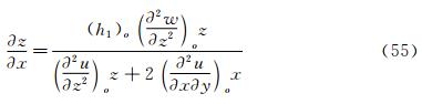
Based on the critical point theory, we know that the point ‘o’ is a saddle on the cross section perpendicular to the separating line if
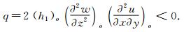
As q>0, ‘o’ is a node or a focus. Because on the separating point the flow leave the wall, which means w>0,  >0, and
  >0 if q>0. Hence
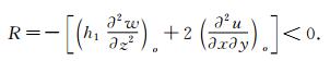
Due to the instability of node and focus point, the possible pattern of ‘o’ is a saddle where <0. And we can obtain a criterion of separation:
Further studies on the separation line showed that: 1) the separation line is a limiting streamline, not an envelope of limiting streamline. Limiting streamline in the near region will converge toward it. 2) There are two possible starting points for the separation line. One is regular point and the second is a saddle point. The separation line started from a regular point is of open type. On the other hand, the separation starting from a saddle point is a closed type. Fig. 11 is the possible pattern of flow separation.
 |
| Fig. 11 Possible pattern of separation. |
Similar analysis for the flow separation described by boundary layer equation show that the separation line is the envelope of limiting streamline due to the Goldstein singularity [9].
Wang [44] pointed out that the above study on flow separation settle down the long-standing dispute regarding whether the separation line is an envelope of the limiting streamlines or the skin friction lines, or if it is also a limiting streamline. This question has since been clarified by Zhang (1985) who concluded that both versions are partly correct, i.e. the separation line is an envelope if based on the boundary layer theory, but it is a limiting streamline if based on the Navier-Stokes equations.
4.2 Body Surface Flow TopologyBecause formula (50) is valid at any point on the body surface, substituting (50) into (54) neglecting high order terms and considering z→0, we can obtain
It describes the limiting streamlines to the body surface. Now, we consider the singular point “S” which satisfies  =
= =0.
=0.
To define J= 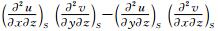 and q= -
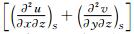 , we can obtain following conclusions based on the nonlinear analytical theory:
1) If J>0, 4J-q>0 and q>0, the point “S” is a stable node of limiting streamline. If J>0, 4J-q>0 and q<0, the point “S” is an unstable nodal.
2) If J>0, 4J-q<0 and q>0, the point “S” is a stable node of limiting streamline. If J>0, 4J-q<0 and q<0, the point “S” is an unstable node.
3) If J<0, the point “S” is a saddle.
4) If J>0, 4J-q<0 and q=0, Hopf bifurcation will undergo at the point “S”. When q changes its sign from q>0 through q=0 to q<0, there is a stable limit cycle. As q changes its sign from q<0 through q=0 to q>0, there is an unstable limit cycle.
5) On the body surface, Lighthill have proved that
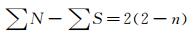
Where ΣN is the number of nodes. ΣS is the number of saddles. And n is the degree of surface connection. For a single connected region, n=1. For a double connected region, n=2.
4.3 Cross-flow Topology [47, 48]As we study the property of flow separation on body surface, it is necessary to study the spatial characteristic of flow structure. Supposing x, y , z are the orthogonal coordinate system with z being the axis of body, x laying on the configuration line which is intersection line of body surface with transverse plane normal to z-axis, and y-axis being normal to the configuration line outwards. u, v, w are the velocity components along x, y, z direction respectively. Using the qualitative theory of the ordinary differential equation, we analyzed the patterns of the sectional streamlines in the transverse planes. The following topological rules can be obtained [47]:
1) When the angle between the body surface and its axis is not zero, the configuration line is not a sectional streamline. If this configuration line does not pass through a singular point of limiting streamlines on the body surface, there are no singular point of sectional streamlines on it. Otherwise, if the configuration line pass through a singular point of limiting streamlines on body surface, this point is also a singular point of the sectional streamlines (called as half singular point) and their behavior of singularity are the same. When the angle between the body surface and its axis is zero, the configuration line is a sectional streamline. If this configuration line passes through a singular point of limiting streamlines on the body surface or the configuration line is normal to the limiting streamline, then this point is a singular point of the sectional streamline.
2) In the transverse plane of the body, the number of singular points of sectional streamlines agrees the following law:
Where Ic is Poincare index along the closed curve C of the above configuration line. ΣN, ΣS is the number of nodal and saddle points in the field outside curve C. ΣN′, ΣS′ is the number of half-nodal and half-saddle points on the curve C.
3) We can prove that Ic=1 if the transverse plane is located in region where no reverse flow along the main streamline direction existed. However, in the case that the transverse plane is located in the reverse flow region on body surface, Ic=0. This means that the change of Poincare index along the longitudinal direction can tell us the information about the longitudinal separation. Hence the longitudinal separation criterion is: ahead of the longitudinal separation region Ic=1. In the longitudinal separation region Ic=0. Behind longitudinal separation region, Ic=1. The change of Ic from 1 to 0 and from 0 to 1 indicates the beginning and the end of the longitudinal separation respectively.
4) Supposing configuration line is symmetric and A, B are the points on upwind and lee side respectively. When  >0(<0), the number of the singular points is the odd (even). When
  >0(<0), the number of the singular points is the even (odd).
The theory of flow separation in the subsections 4.1 and 4.2 was verified [9, 48, 49, 50] through physical analysis and numerical simulation. For example, He G H and Li Z W [9] simulated the hypersonic flow over a capsule type body and space shuttle like configuration, which are shown in Figs. 11 and 12 for the surface flow and cross flows in different transversal planes. Different patterns of flow separation were obtained and agree with the analysis.
 |
| Fig. 12 Surface flow and cross flows for a capsule configuration. |
 |
| Fig. 13 Spatial flow structure of a space shuttle-like configuration. |
In addition, applying the theory of structural stability [51, 52] in mathematics, Zhang and Ran developed the structural stability of velocity fields [53, 54]. It is pointed out that as there is a sectional streamline connecting two saddle points in the symmetric line shown in Fig. 14 (c), the symmetric flow field loses its stability.
 |
| Fig. 14 Changed flow fields at different angles of attack for hypersonic flow over slender body M∞=10, Re=1×10⁵. |
Fig. 15 shows the velocity distribution at lee-ward symmetrical line and sectional streamlines, which agree with the theoretical analysis. As the angle of attack α=12°, there is two saddle points on symmetric line of lee side. Then the loss of flow structure stability begins with this angle attack increased.
 |
| Fig. 15 Velocity distribution at lee-ward symmetrical line (left) and sectional streamlines for hypersonic flow over slender body M∞=10, Re=1×10⁵. |
From 1992, Zhang [55, 56] studied the flow pattern of vortex in the cross section perpendicular to the vortex. He obtained the evolution of vortex structure on the cross section perpendicular to the vortex axis and found that there is Hopf bifurcation in the sectional streamlines. As a result, there is a limit cycle in the sectional streamlines. Moreover, there is an essential difference between a subsonic vortex and a supersonic vortex.
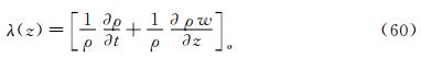
Suppose x, y and z are three axes of an orthogonal coordinate system, (u, v, w)is velocity components in the directions of x, y and z respectively. z is in the vortex axis. x, y locate on the cross section perpendicular to the vortex axis. The equation to describe the sectional streamline on the cross section perpendicular to the vortex is
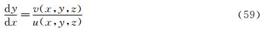
Using the boundary condition on the vortex axis and critical point theory, we can obtain the function λ(z) that determines the pattern of the sectional streamlines for NS equations. The function λ(z) has the following form:
where, ρ is density and subscript “o” shows a point on the axis of vortex. For steady flow:
The analysis concluded that:
1) If λ(z) > 0, the sectional streamline in the cross section perpendicular to the vortex axis spiral inward in the near region of the vortex axis.
2) If λ(z)<0, the sectional streamline in the cross section perpendicular to the vortex axis spiral outward in the near region of the vortex axis.
3) If λ(z) changes sign along the vortex axis, Hopf bifurcation will occurs, which results in a limit cycle in the section streamlines.
Using the NS equation, λ(z) can be written as
where M and p is Mach number and pressure respectively. ε(1/Re) represents the viscous term. When Reynolds number Re>>1, ε(1/Re) can be neglected. It is shown that there is an essential difference between a subsonic vortex case and a supersonic vortex one along the axis-z. For a subsonic swirling flow, the sectional streamlines in the vicinity of the vortex axis spiral inwards in the locally favorable pressure region and they spiral outwards in the locally adverse pressure region. However, for a supersonic swirling flow, the sectional streamlines in the vicinity of the vortex axis spiral outwards in the locally favorable pressure region and they spiral inwards in the locally adverse pressure region.
Fig. 16 represents the relationship between the function λ(z) and the vortex structure. Based on the found of limit cycle, Zhang H X proposed a concept of “Black hole” in vertical flow, which was proved by Zhang [57] through numerical simulation of the vertical flow over a Delta wing, which is shown in Fig. 17 for the trajectories starting from the apex.
 |
| Fig. 16 Relationship between the function and the vortex pattern in the cross section perpendicularto the vortex axis. |
 |
| Fig. 17 Black hole in the lee-side of a delta wing. |
The above theory on the steady vertical flow was proved by Zhang [57] and Chen [58] and was extended to unsteady flow by Zhang et al. [59]. A similar function λ(z, t) of was obtained to determine the sectional streamlines pattern for unsteady flow. The interaction of a normal shock wave and a longitudinal vortex was simulated. Fig. 18 is the variation of λ(z, t) along the vortex axis at typical instant t=11. Fig. 19 contains the sectional streamlines at several typical cross sections. The numerical result agrees with the theoretical result. One more limit cycle is observed when λ(z) changes its sign.
 |
| Fig. 18 Distribution of λ on the vortex axis at t=11. |
 |
| Fig. 19 Sectional streamline pattern in the cross-section perpendicular to the vortex axis t=11. |
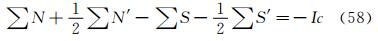
When the vehicle is in pitching oscillation, the coupled equations describing the pitching oscillations of the vehicle and the unsteady flow around it are [60]:

The first equation describes the single-freedom pitching motion of the capsule about its center of gravity. I is the dimensionless rotation inertia. Cm and Cμ are coefficients of the pitching moment and the damping moment. Note that Cμ in free flight is zero, but it must be considered in wind tunnel experiments.  and
and  are the first and the second order temporal derivatives of θ. The second equation is the unsteady Navier-Stokes equation. The third equation is the integration formula of pitching moment coefficient, where r is the vector from the point on the body surface to the center of gravity. k is the unit vector in the direction of axis z, n and τ are unit vectors on the body surface in normal and tangential directions respectively. pn and σ are stresses on the body surface in the normal and tangential directions respectively.
 , we can obtain the nonlinear dynamic system to describe the pitching motion as:
where
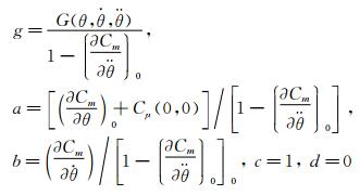
With the dynamics system (65), we can analyze the property of the vehicle in the near region of the trim point. There are three different cases. The first is that it has only one trim point. The second has two trim points and the third has three trim points. Next, we will analyze them separately.
4.5.1 Qualitative Property of the Dynamic System Having One Trim PointIn the case (∂Cm/∂θ)0<0, there is one trim point. The condition of dynamic stability for the nonlinear system could be written as
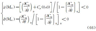
Sometimes, the second condition could also be written as
This condition is stricter, which requires the phase portrait of the stable motion to be the spiral point. If Eq. (66) is not satisfied, the motion is dynamically unstable. Stable and unstable states are shown in Figs. 20 and 21.
 |
| Fig. 20 State of λ<0 and Δ<0. |
 |
| Fig. 21 State of λ>0 and Δ>0. |
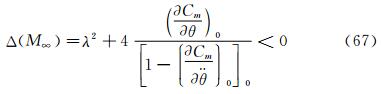
Moreover, the characteristic values of the Jacobian matrix of the linear parts of Eq. (65) are two unequal roots: ω1, 2=  . At λ=λ cr =0, following conditions are satisfied:
1) The real part of the characteristic values: Re[ω1(λ cr ), ω2(λ cr )]=0.
2) The imaginary part of the characteristic valuse: Im[ω1(λ cr ), ω2(λ cr )]=0
3) 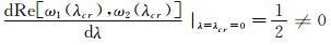
Therefore the characteristic values of the system satisfy the three conditions of Hopf bifurcation at λ=λcr=0. This indicates that Hopf bifurcation would happen for a nonlinear dynamic system when λ changes from λ<0 to λ=0. On the (x, y) phase plane, a stable limit cycle would occur (Fig. 22(a)). The time history curve of pitching oscillation angle would present a periodic oscillation (Fig. 22(b)).
 |
| Fig. 22 State of λchanges from λ<0 through λ>0 to λ>0. |
Here, we theoretically obtain the critical condition of the happening of Hopf bifurcation as well as the occurrence of the limit cycle:
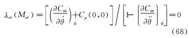
from which the critical Mach number could be determined.
4.5.2 Qualitative Analysis of the Dynamic System Having Two Trim Points on the Moment CurveWhen the Mach number decreases from a high number to a certain number, the moment curve changes from having one trim point to two trim points. For critical case which changes from having one trim to two trim points, we can prove that it is dynamic instability and is saddle node bifurcation.
4.5.3 Phase Portrait in the Neighborhood of the Three Trim Points at M∞<McrWhen Cμ=0, (∂Cm/∂θ) 0 <0, >0 and <0 are respectively at the three trim points α1, α2 and α3 of Eq. (65). So α1 and α3 are nodal points while α2 is a saddle point. The form of the α- phase portrait is different with respect to the difference of (∂Cm/∂θ) 0. For example, when (∂Cm/∂θ) 0 < 0 at α1 and α3 respectively, the phase portrait at α1 and α3 are all stable nodals (Fig. 23).
 |
| Fig. 23 Phase portrait structure of Δ<0 respectively at α1 and α3. |
Chinese CFD got its great development in the past thirty years. NND scheme was a milestone in Chinese CFD, which has been extensively applied to flow mechanism study and numerical simulations of engineering problems with complex configurations. Moreover, there were many landmarks, such as the five Ms and one A , the four principles to design numerical scheme.
The key creative idea of Chinese CFD is emphasizing the coupling study of the computational fluid dynamics and physical analysis. Based on the powerful tool of CFD, a lot of mechanisms of fluid mechanics were revealed including the steady and unsteady flow separation, vortex motion, dynamic derivatives for vehicle and the generation of aerodynamic noise.
However, there are still many grand challenges in CFD. With the fast development of supercomputer and high order numerical schemes in recent years, we believe that it is the best time for CFD to reveal the detail fluid mechanisms for multi-scale problems, such as turbulence and aeroacoustics.
It should be pointed out that this paper does not contain everything of CFD in China due to the space limitation. The authors would like to show sorry on this regard.
Acknowledgment: The authors appreciate Professors Shen M Y, Fu D X and Li X L for their contribution to both the development of Chinese CFD and the writing of this paper.
| [1] | Xu J H, Gu F Z. HLHL Prize, the selection board of Ho Leung Ho Lee foundation[M]. Beijing:China science & technology press, 1997. |
| [2] | Zhang H X. The exploration of the spatial oscillations in finite difference solutions for Navier-Stokes Shocks[J]. Acta Aerodynamica Sinica, 1984,1(1):12-19.(in Chinese) |
| [3] | Zhuang F G, Zhang H X. Review and prospect for computational aerodynamics[J]. Advances in Mechanics, 1983, 13:2-18. |
| [4] | Zhang H X, Zhang L P, Zhang S H, et al. Some recent progress of high-order methods on structured and unstructured grids in CARDC[C]//The eighth international conference on computational fluid dynamics, 7, 14-18, 2014, Chengdu, China. |
| [5] | Zhang H X. Non-oscillatory and non-free-parameter dissipation difference scheme[J]. Acta Aerodynamica Sinica, 1984,6(2):143-165. |
| [6] | Zhang H X, Zhuang F G. NND schemes and their applications to numerical simulation of two and three dimensional flow[J]. Advances in Applied Mechanics, 1991, 29:193-256. |
| [7] | Zhang H X, Shen M Y. Computational fluid dynamics-fundamentals and applications of finite difference methods[M]. Beijing National defense industry press, 2002. |
| [8] | Zhang L P. Numerical simulations for complex inviscid flow fields on unstructured grids and Cartesian/unstructured hybrid grids[D]. Mianyang:China Aerodynamics Research and Development Center, Ph.D. Thesis, 1996. |
| [9] | He G H. Third-order ENN scheme and its application to the calculation of complex hypersonic viscous flows[D]. Mianyang:China Aerodynamicscs Research and Development Center, Ph.D. Thesis, 1994. |
| [10] | Shen Q. Numerical simulation of three dimensional complex viscous hypersonic flow[D]. Mianyang:China Aerodynamicscs Research and Development Center, Ph.D. Thesis, 1991. |
| [11] | Deng X G. Numerical simulation of viscous complex supersonic flow interaction[D]. Mianyang:China Aerodynamicscs Research and Development Center, Ph.D. Thesis, 1991. |
| [12] | Zong W G, Deng X G, Zhang H X. Double weighted essentially nonoscillatory shock capturing schemes[J]. Acta Aerodynamica Sinica, 2003, 21(2):218-225. |
| [13] | Li Q. The difference schemes of high order accuracy, boundary processing methods and the numerical simulation on planar mixing layer[D]. Mianyang:China Aerodynamicscs Research and Development Center, Ph.D. Thesis, 2003. |
| [14] | Zhang L P, Zhao Z, Chang X H, He X. A 3D hybrid grid generation technique and multigrid/parallel algorithm based on anisotropic agglomeration approach[J]. Chinese Journal of Aeronautics, 2013, 26(1):47-62. |
| [15] | Heim E R. CFD wing/pylon/finned store mutual interference wind tunnel experiment[R]. Eglin Air Force Base, FL 32542-5000, February, 1991. |
| [16] | Shen M Y, Niu X L, Zhang Z B.The properties and applications of the generalized compact scheme satisfying the principle about suppression of the oscillations[J]. Chinese Journal of Applied Mechanics, 2003, 20:12-20. (in Chinese) |
| [17] | Zhang Z C, Li H D, Shen M Y. Space-time conservation schemes for 3-D Euler equations[C]//Proceeding seventh international symp on CFD. Beijing China, 1997:259-262. |
| [18] | Fu D X, Ma Y W. A high order accurate difference scheme for complex flow fields[J]. Journal of Computational Physics, 1997, 134:1-15. |
| [19] | Ma Y W, Fu D X. Fourth order accurate compact scheme with group velocity control[J]. Science in China, 2001, 44:1197-1204. |
| [20] | Deng X G, Mao M L, Liu H Y, et al. Developing high order linear and nonlinear schemes satisfying geometric conservation law[C]//The eighth international conference on computational fluid dynamics. 2014, Chengdu, China. |
| [21] | Deng X G, Maekawa H. Compact high-order accurate nonlinear schemes[J]. J. Comput. Phys., 1997, 130(1):77-91. |
| [22] | Deng X G, Zhang H X. Developing high-order weighted compact nonlinear schemes[J]. J. Comput. Phys., 2000, 165:22-44. |
| [23] | Zhang S H, Jiang S F, Shu C W. Development of nonlinear weighted compact schemes with increasingly higher order accuracy[J]. J. Comput. Phy., 2008, 227:7294-7321. |
| [24] | Liu X L, Zhang S H, Zhang H X et al. A new class of central compact schemes with spectral-like resolution I:Linear schemes[J]. J. Comput. Phys., 2013, 248:235-256. |
| [25] | Liu X L, Zhang S H, Zhang H X, et al. A new class of central compact schemes with spectral-like resolution II:Hybrid weighted nonlinear schemes[J]. J. Comput. Phys., 2015, 284:133-154. |
| [26] | Zhang S H, Jiang S F, Shu C W. Improvement of convergence to steady state solutions of Euler equations with the WENO schemes[J]. Journal of Scientific Computing, 2011, 47:216-238. |
| [27] | Zhang S H, Shu C W. A new smoothness indicator for the WENO schemes and its effect on the convergence to steady state solutions[J]. Journal of Scientific Computing, 2007, 31, Nos. 1/2:273-305. |
| [28] | Zhang L P, Liu W, He L X, Deng X G, Zhang H X. A class of hybrid DG/FV methods for conservation laws I:Basic formulation and one-dimensional systems[J]. J. Comput. Phys., 2012, 231:1081-1103. |
| [29] | Zhang L P, Liu W, He L X, et al. A class of hybrid DG/FV methods for conservation laws II:Two-dimensional Cases[J]. J. Comput. Phys., 2012, 231:1104-1120. |
| [30] | Zhang L P, Liu W, He L X, Deng X G, Zhang H X. A class of hybrid DG/FV methods for conservation laws III:Two-dimensional Euler equations[J]. Comm. Comput. Phy., 2012, 12(1):284-314. |
| [31] | Zhang L P, Liu W, He L X, et al. A class of DG/FV hybrid schemes for conservation law IV:2D viscous flows and implicit algorithm for steady cases[J]. Computers & Fluids, 2014, 97:110-125. |
| [32] | Zhang S H, Li H, Liu X L, et al. Classification and sound generation of two-dimensional interaction of two Taylor vortices[J]. Physics of Fluids, 2013, 25:056103. |
| [33] | Zhang S H, Jiang S F, Zhang Y T, et al. The mechanism of sound generation in the interaction between a shock wave and two counter rotating vortices[J]. Phys. Fluids. 2009, 21(7):076101. |
| [34] | Zhang S H, Zhang Y T, Shu C W. Interaction of an oblique shock wave with a pair of parallel vortices:Shock dynamics and mechanism of sound generation[J]. Phys. Fluids. 2006, 18(12):126101. |
| [35] | Zhang S H, Zhang Y T, Shu C W. Multistage interaction of a shock and a strong vortex[J]. Phys. Fluids. 2005, 17(11):116101. |
| [36] | Li X L, Fu D X, Ma Y W. Direct numerical simulation of compressible isotropic turbulence[J]. Science in China A, 2002, 45(11):1452-1460. (in Chinese) |
| [37] | Fu D X, Ma Y W, Zhang L B. Direct numerical simulation of transition and turbulence in compressible mixing layer[J]. Science in China A, 2000, 43(4):421-429.(in Chinese) |
| [38] | Gao H, Fu D X, Ma Y W, et al. Direct numerical simulation of supersonic boundary layer[J]. Chinese Physics Letter, 2005, 22(7):1709-1712. (in Chinese) |
| [39] | Li X L, Fu D X, Ma Y W. Direct numerical simulation of a spatially evolving supersonic turbulent boundary layer at Ma=6[J]. Chinese Physics Letters, 2006, 23(6):1519-1522. |
| [40] | Li X L, Fu D X, Ma Y W. Direct numerical simulation of hypersonic boundary-layer transition over a blunt cone[J]. AIAA Journal, 2008, 46(11):2899-2913. |
| [41] | Li X L, Fu D X, Ma Y W. Direct numerical simulation of hypersonic boundary layer transition over a blunt cone with a small angle of attack[J]. Physics of Fluids, 2010, 22:025105. |
| [42] | Li X L, Fu D X,Ma Y W, et al. Direct Numerical Simulation of Shock/Turbulent Boundary Layer Interaction in a Supersonic Compression Ramp[J]. Science China:Physics, Mechanics & Astronomy, 2010, 53(9):1651-1658.(in Chinese) |
| [43] | Zhang H X, Guo C, Zong W G. Problems about grid and high order schemes[J]. Acta Mechanica Sinica, 1999, 31(4):398-405. |
| [44] | Wang K C, Zhou H C, Hu H C, et al. Three-Dimensional Separated Flow Structure over Prolate Spheroids[J]. Proceedings of the Royal Society of London. Series A, Mathematical and Physical Sciences. 1990, 429:73-90. |
| [45] | Zhang H X. The separation criteria and flow behavior for three dimensional steady separation flow[J]. Acta Aerodynamica Sinica, 1985, 1(1):1-12. (in Chinese) |
| [46] | Zhang H X. The behavior of separation line for three dimensional steady viscous flow-based on boundary layer equations[J]. Acta Aerodyn. Sin, 1985, 4(1):1-8. (in Chinese) |
| [47] | Zhang H X. Crossflow topology of three dimensional separated flows and vortex motion[J]. Acta Aerodynamica Sinica, 1997, 15(1):1-12.(in Chinese) |
| [48] | Zhang H X, Guo Y J. Topological flow patterns on cross section perpendicular to surface of revolutionary body[J]. Acta Aerodynamica Sinica,2000, 18(1):1-13. |
| [49] | Li Z W, Numerical simulation for the complex hypersonic flow with shock waves, vortices and chemical action[D]. Mianyang:China Aerodynamicscs Research and Development Center, Ph.D. Thesis, 1994. |
| [50] | Guo Y J. Numerical/analysis investigation of hypersonic flowsover a blunt cone with and without spin[D]. Mianyang:China Aerodynamicscs Research and Development Center, Ph.D. Thesis. 1997. |
| [51] | Peixoto M M. On structural stability[J]. Annu. Math, 1959, 69:199-222. |
| [52] | Peixoto M M. Structural stability on two-dimensional manifolds[J]. Topology, 1962, 1:101-120. |
| [53] | Zhang H X, Ran Z. On the structure stability of the flows over slenders at angle of attack[J]. Acta Aerodynamica Sinica, 1997, 15(1):20-26.(in Chinese) |
| [54] | Ran Z. Structure stability analysis and numerical simulation of flows over slender cones[D]. Mianyang:China Aerodynamicscs Research and Development Center, Ph.D. Thesis. 1997. |
| [55] | Zhang H X. The evolution of nonlinear bifurcation of vortex along its axis[R]. Mianyang:China Aerodynamicscs Research and Development Center report. 1992. |
| [56] | Zhang H X. The topological analysis of subsonic and supersonic vortex[R]. Mianyang:China Aerodynamicscs Research and Development Center Report. 1994. |
| [57] | Chen J Q. Numerical simulation of supersonic combustion and vortex motion[D]. Mianyang:China Aerodynamicscs Research and Development Center, Ph.D. Thesis. 1995. |
| [58] | Zhang S H. Numerical simulation of vertical flows over delta wings and analysis of vortex motions[D]. Mianyang:China Aerodynamicscs Research and Development Center, Ph.D. Thesis. 1995. |
| [59] | Zhang S H, Zhang H X, Shu C W. Topological structure of shock induced vortex breakdown[J]. Journal of fluid mechanics. 2009, 639:343-372. |
| [60] | Zhang H X, Yuan X X, Liu W, et al. Physical analysis and numerical simulation for the dynamic behavior of vehicles in pitching oscillations or rocking motions[J]. Science in China Series E:Technological Sciences. 2007, 50:1-17. |