 2017, Vol. 60


2 Jiading District Meteorological Bureau, Shanghai 201821, China
The planetary boundary layer (PBL) is the bottom layer of the troposphere, and is closest to the underlying surface. The thickness of the PBL is several hundred meters to 1~2 kilometers. Because of the influence of the underlying surface, the PBL shows significant turbulence characteristics. The turbulence intensity, as well as the thickness of the boundary layer plays an important role in transporting atmospheric momentum, heat, water vapor and pollutants, which affects the weather and climate changes. Therefore, in-depth study of the atmospheric boundary layer and the atmospheric turbulence is essential to human healthy life.
At present, the study of the PBL is mainly carried out by field observations and numerical simulations. WRF (Weather Research and Forecasting) plays an important role in the research of small scale, mesoscale and large scale weather system simulations. However, in the model WRF, the horizontal and vertical resolutions are usually set to above 1 km, which means that the resolution is coarse. In contrast to that, the atmospheric turbulence motion belongs to the sub-grid scale motion thus cannot be calculated directly. Therefore, the only way to describe the sub-grid scale turbulence on mesoscale meteorological elements is to use the parameterization schemes (Shin et al., 2011). With the continuous development of numerical simulation technology, different PBL parameterization schemes have been developed. The main difference among those schemes is the turbulence closure, which leads to different vertical diffusion rate of the momentum, heat and water vapor, and as well as the simulation results of the PBL. In total, there are 12 PBL parameterization schemes in the present WRF model. Each parameterization scheme has different applicability and limitation due to the treatment methods of the turbulence. Thus, the simulated results are different under different conditions, such as different weather, underlying surface and seasons. Among them, the most commonly used PBL schemes are ACM2 (Asymmetric Convective Model version 2) (Pleim, 2007), YSU (Yonsei University) (Hong et al., 2006), BouLac (Bougeault-Lacarrere) (Bougeault and Lacarrere, 1989), MYJ (Mellor-Yamada-Janjic) (Janjić et al., 1990) and MYNN2.5 (Level 2.5 Mellow-Yamada Nakanishi Niino) (Nakanishi and Niino, 2004).
Many sensitivity tests were performed by using the different PBL parameterization schemes in WRF model to evaluate those schemes in a certain area. For the temperature simulation, the study of Qiu et al. (2013) and Huang et al. (2014) showed that the ACM2 and YSU schemes are better when simulating the alpine steppe areas in the Tibetan Plateau and the forest areas in the northern United States. A study of the hilly terrain in the Loess Plateau indicated that the YSU scheme is better when simulating at day time, and the MYJ scheme is better at night time (Wang et al., 2013). For the wind speed, Wang et al. (2010) and Zhang and Yin (2013) found that ACM2 scheme performs better in the urban area of Lanzhou and Huangshan of Anhui province in winter. Kim et al. (2013) noted that YSU and MYNN2.5 are superior in urban and suburban areas of Paris. For the sensible and latent heat, a study suggested that the MYJ scheme is better when simulating the sensible heat and the ACM2 scheme is better when simulating the latent heat in the northwestern mountains in winter (Zhang, 2012). A study by Qiu et al. (2013) showed that the MYNN2.5 scheme is better when simulating the alpine steppe of Tibetan Plateau. Therefore, under different conditions, the simulated results of the PBL parameterization schemes are uncertain. More evaluation of the parameterization schemes based on more representative cases is highly demanded for the improvement and development of the PBL parameterization schemes.
However, the studies mentioned above are usually conducted for the clear days. The studies on the performance of PBL parameterized schemes under cloudy or overcast days are still lacking. The existence of the cloud affects the simulated results of the meteorological elements with different PBL parameterization schemes. Hu et al. (2010) found in the simulated results in Huston areas that, the maximum temperature error is very little on some days but with more substantial cold biases on the other days, and they suggested that this day time temperature bias may be caused by the errors in cloud cover.
In this paper, WRF model combined with a long-term observational data for the typical farmland in Shouxian County, Anhui, provided by the US Department of Energy's Observatory of Atmospheric Radiation Observations (ARM) mobile observation stations, were used to simulate the meteorological elements and the PBL structure in the clear and the overcast conditions. The simulated results of 5 different PBL parametrization schemes (ACM2, BouLac, MYJ, MYNN2.5 and YSU) were also evaluated, which provides a scientific reference for the selection of the boundary layer parameterization scheme in the clear and the overcast conditions.
2 MODEL CONFIGURATION AND EVALUATION DATA 2.1 Five PBL Parameterization SchemesThere are two types of PBL schemes: non-local closure schemes such as ACM2 and YSU, and local closure schemes as BouLac, MYJ and MYNN2.5 which we discuss in the following text.
In the PBL schemes, the relationship between the sub-grid disturbance flux 
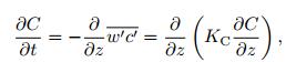
|
(1) |
where KC (Km, Kh and Kε, hereinafter collectively referred to as KC) is the turbulent diffusion coefficient. Every other PBL parameterization schemes are modified on the basis of this equation.
(1) The turbulence closure equation of ACM2 scheme is as follows:

|
(2) |
Mu is the upward non-local convective mixing rate from model bottom; Mdi is the downward non-local mixing rate from the ith layer to the (i -1) th layer; Δzi is the thickness of the model layer; KC is the turbulent diffu-sion coefficient, which is obtained by using turbulent similarity theory and turbulent exchange under different stability conditions. fconv is used to control the proportion of non-local and local effects, fconv = 0 for local mixing, fconv = 1 for non-local mixing. The left side of the equation represents the change in the mean amount over time, the first three terms on the right indicate the non-local mixing due to large scale turbulence, and the fourth term represents the local effect caused by the turbulent exchange.
(2) The turbulence closure equation of YSU scheme is as follows:
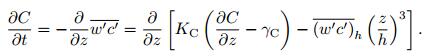
|
(3) |
The anti-gradient flux term γC increases the non-local effects caused by large-scale turbulent vorticity, the entrainment flux term 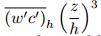
(3) The turbulence closure of the local schemes (BouLac, MYJ, MYNN2.5) is obtained by using the turbulent kinetic energy (TKE) prediction equation:
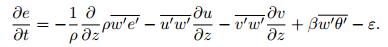
|
(4) |
In Eq.(4), e is the turbulent kinetic energy, u′, v′, w′ is the horizontal and the vertical perturbation velocity, θ′ is the perturbation temperature, β is the buoyancy coefficient and ε is the dissipation rate of the turbulent kinetic energy. The first term on the right side of the equation represents the TKE of turbulent transport, the second and the third terms represent the TKE caused by the wind shear. The fourth and the fifth terms represent TKE dissipation by buoyancy and molecular diffusion, respectively. In Eq.(4),

|
(5) |
The turbulent diffusion coefficient KC = le1/2Sc, where l is the mixing length and Sc is the proportional coefficient. The value of KC is dominant in these three local schemes. As a result, the difference of l and Sc are critical factors which affect the final simulated results.
2.2 Model ConfigurationsIn this paper, the WRF version 3.4 model is used to simulate the Shouxian area of Anhui Province. September 27th to 30th, 2008 are selected for the overcast cases. August 19th, November 12th, November 14th and December 16th, 2008 are selected for the clear cases.
The National Centers for Environmental Prediction (NCEP) global forecast system (GFS) final (FNL) operational global analyses are used for initial conditions and boundary conditions. Three model domains are applied and the simulated center is located at 32.56°N and 116.78°E. The nested grid number and lattice spacing are 114×114 (9 km), 124×124 (3 km) and 154×154 (1 km), respectively. The type of the underlying surface of the simulated area is farmland. All model domains have 50 vertical layers, and there are 28 layers in the lowest 2 km, in order to clearly represent the vertical structure of the PBL. The physical parameterization scheme used in all model domains includes Morrison microphysical scheme, rrtmg long-wave radiation scheme, rrtmg short-wave radiation scheme and Noah land surface scheme. A cumulus scheme is switched off on the 1 km fine domain, while the 9 km and 3 km fine domain use Kain-Fritsch scheme.
2.3 Evaluation DataThe observational data for the comparative evaluation of the model were provided by the U.S. Department of Energy's Atmospheric Radiation Measurement Mobile Observatory, which was obtained in a four-month field campaign at Shouxian, Anhui Province from September to December 2008. The station is located in the Huaihe River Basin, which is an open flat terrain, and is a typical farmland. The observational instruments used in the campaign are comprehensive which can reflect the meteorological characteristics of the farmland in Shouxian, and provide convincing data for the verification (Fan et al., 2010; Lu, 2014). In this campaign, the height of cloud base was detected, the radiation was measured by radiometer, the meteorological elements were measured by ground-based meteorological instruments, the fluxes were measured by vorticity correlation instrument, and the vertical profiles of meteorological elements were detected by GPS radiosonde. The underlying surface of the simulated area is flat and uniform, the distribution of meteorological elements is uniform, and the output data represent the status of the grid center. Therefore, a five-point-averaged method is applied to reduce the systematic errors (Huang et al., 2014; Gibbs, 2011).
3 RESULTS AND DISCUSSION 3.1 Comparison of the Cloud CharacteristicsAccording to the satellite infrared cloud diagram (not shown here), from September 27th to 30th, 2008, there is a continuous large-scale cloud system over Anhui Shouxian area. The ground-based observational data of Shouxian also shows that these four days are overcast days. The cloud amount in the simulated center area was 10, and the surface temperature was 16 ℃~24 ℃. Moreover, the relative humidity was 45%~90%, and the precipitation was not detected. Besides, the wind is mainly north wind, and the wind speed was ranging from 3 to 6 m·s-1. By using the ceilometer and GPS radiosonde, the simulated results of 5 PBL parameterization schemes for four overcast days were compared and analyzed. The GPS radiosonde uses the relative humidity profile to determine the cloud. When the relative humidity is larger than 95%, it is considered as the existence of cloud. In the WRF model, the threshold of the existence of cloud is defined as Q = QCLOUD+QICE > 0.01 g·kg-1 (Rachel et al., 2013).
Figure 1a shows the height of the cloud base measured by ceilometer from Sep. 27th to Sep. 30th. Fig. 1b to 1f show the profiles of time and height of the five schemes. The ceilometer shows there are cloud all day on Sep. 27th, the height of cloud base was about 2000 m, GPS radiosonde also shows the cloud thickness of 800~1000 m. All the 5 schemes failed to simulate the existence of the cloud at night time. The simulated result of the cloud base at the day time is all about 2200 m by these 5 schemes, where the thickness of cloud layer simulated by the three local schemes varies a lot, while the thickness of the two non-local schemes are about 1000 m, which are more uniform and closer to the observational result. The ceilometer shows that the cloud base on Sep. 28th was 1500~2000 m, the GPS radiosonde shows the cloud thickness was 500~1000 m. All the simulated results of the height of cloud base by these 5 schemes are about 2200 m. The result of BouLac scheme is discontinuous. In contrast, the simulated results of the other 4 schemes are more uniform and the thicknesses of the cloud are all about 800 m, which are closer to the observational result. The ceilometer shows that clouds exist on Sep. 29th except at noon, and the height of the cloud base is 1500~2000 m. The GPS radiosonde shows the thickness of cloud is 500~800 m. Three local schemes failed to simulate the condition of the cloud which differed a lot from the observational result. However, the cloud base height (2200 m), the cloud thickness (500 m), as well as the no-cloud condition at noon are simulated by the non-local schemes ACM2 and YSU, which are closer to the observational result. The ceilometer does not detect any cloud from 08:00 to 12:00, in the rest of the time exist clouds on Sep. 30th, and the height of the cloud base is 2000 m. GPS radiosonde shows that the clouds are thin. All the simulated results of the cloud base height of 5 schemes are 1500 m, which is 500 m lower than the observation, and they can only simulate the cloud condition during 12:00–18:00, and there are some deviations from the observational results. Overall, non-local schemes (ACM2 and YSU) perform better than the local schemes (BouLac, MYJ, and MYNN2.5) in simulating the cloud base height, the cloud thickness, and the cloud lifetime. A large amount of vapor is transported to the upper layer from the ground due to the strong non-local effects of the ACM2 and YSU schemes. Thus, the humidity reaches the threshold value of cloud in the model. Dry air is entrained into the air at high altitude so that the thickness of the cloud is not too thick and is closer to the observed value. Even if the microphysics schemes are the same, different PBL schemes still have a great impact on cloud simulations by influencing the vertical transport of the vapor.

|
Fig. 1 The comparison of the clouds in the Shouxian between the observed and the simulated with different PBL scheme from Sep. 27th to Sep. 30th, 2008 (a) Ceilometer; (b) BouLac scheme; (c) MYJ scheme; (d) MYNN2.5 scheme; (e) ACM2 scheme; (f) YSU scheme. |
By comparing the daily variation of mean temperature at 2 m height in clear days and overcast days, we were able to see that all the 5 PBL schemes can simulate the daily variation of the temperature at 2 m height well. Fig. 2a shows that the simulated values of day time are lower than the observations, while the simulated results of night time are higher. Therein, the non-local schemes ACM2 and YSU have higher simulated result at day time and lower at night time than the local schemes, and are closer to the observations. Fig. 2b shows that under overcast conditions, the simulated results of all 5 schemes are higher at day time, and the local schemes have higher simulated temperature than the non-local scheme. Therein, the simulated result of the ACM2 scheme is the closest to the observational result, while the result of the BouLac scheme has the largest deviation from the observational result. At the night time the results of ACM2, MYJ and MYNN2.5 are closer to the observed values, while the simulated values of the other two schemes are higher than the observation. The results of the temperature simulation are mainly affected by two aspects. The first factor is the treatment of the shortwave radiation to the ground in different schemes. The shortwave radiation of the sun is affected by the reflection, the scattering, the absorption and other weakening effect. The second one is the treatment of the turbulence mixing in different schemes. In clear days, the amount of radiation reaching the ground is constant, the deviation caused by the own factors of schemes is small. However in the overcast days, the simulated results of the clouds of the different schemes lead to the differences of the amount of shortwave radiation reaching the ground, which makes the simulation of the 2 m temperature also different. During the day time, the ACM2 scheme simulates the clouds best, so the simulated temperature at 2 m height is also the closest to the observed value. However, the other schemes overestimate the downward shortwave radiation (not shown here), making the simulated surface temperature also overestimated, which cause higher simulated temperature at 2 m height. At the night time, the deviation of all the simulated radiation from observed value can be ignored. Thus, the difference of simulated temperature is mainly caused by the different treatments of the turbulence mixing in each scheme. The non-local scheme YSU, because of its stronger turbulence mixing effect, results in a higher value of the temperature in simulations. In contrast, the ACM2 scheme adjusts the coefficient fconv in the stable condition, to reflect the local characteristics by weaken the non-local characteristics. Therefore, when the night temperature is simulated, the ACM2 scheme is similar with the other three local schemes. Under the clear day condition, the ACM2 scheme performs best, the correlation coefficient is 0.98, and the root mean square error is 1.27. Under the cloudy condition, the ACM2 scheme is also the best, the correlation coefficient is 0.99 and the root mean square error is 0.33.

|
Fig. 2 The comparison of the mean temperature at 2 m height between the observed and the simulated with different PBL scheme during the simulated time (a) Clear day; (b) Overcast day. |
The simulated results of 5 schemes on the daily variation of the mean vapor at 2 m height in clear days and overcast days are compared (Fig. 3). The simulated values of all the 5 schemes are higher than the observed values at the day time, both in clear day and overcast day. Therein, the simulated values of the non-local schemes, ACM2 and YSU, are lower than those of the three local schemes, and are closer to the observations. It is mainly due to the consideration of the non-local transport and the entrainment processes in the non-local schemes, resulting in the transport of near-surface vapor to the upper layer, causing less vapor simulation than the local schemes. During the night time, the differences of the simulated results of all the 5 schemes in the clear days are small. However, the simulated values of each scheme during the overcast days are higher than those during the day time. Therein, the YSU scheme has stronger turbulence mixing ability which causes a higher vapor growth than other schemes. Under the clear day condition, the ACM2 scheme behaves best, the correlation coefficient is 0.99, and the root mean square error is 0.91. Under the overcast condition, the ACM2 scheme is also the best, the correlation coefficient is 0.71 and the root mean square error is 0.58.

|
Fig. 3 The comparison of the mean vapor at 2 m height between the observed and the simulated with different PBL scheme during the simulated time (a) Clear day; (b) Overcast day. |
Figure 4 shows the daily variation of the mean wind speed and wind direction at 10 m height in clear days and overcast days. For the wind speed, the correlation coefficients of the five schemes are small in both clear day and overcast day, which range from 0.21 to 0.45. The root mean square error indicates that the simulated wind speed of all the five schemes is larger than observation. The simulated wind speeds of the local schemes are smaller than that of non-local schemes, and are closer to the observation. Therein the MYJ scheme is the best, and the difference of the correlation coefficient between the simulated results of the MYJ scheme and the wind speed in clear day and overcast day are small (0.45 in clear days and 0.43 in overcast days). However, the error of root mean square under clear day condition is larger than that under overcast condition (1.08 in clear days and 0.43 in overcast days). Thus, the wind speed deviation in clear days is larger. For the wind direction, the deviation of the same scheme under clear day conditions (about 60°) is larger than that of overcast day (about 25°). Therein the MYJ scheme has the best effect in the clear day simulation, the correlation coefficient is 0.36, and the root mean square error is 63.7. The BouLac scheme performs best under overcast conditions, the correlation coefficient is 0.60, and the root mean square error is 9.34. The difference of wind speed and wind direction among different schemes may be caused by the different mixing length and the different friction velocity impacted by the different turbulent diffusion coefficients used in different schemes.

|
Fig. 4 The comparison of the mean wind speed (c) and wind direction at 10 m height between the observed and the simulated with different PBL scheme during the simulated time (a), (c) Clear day; (b), (d) Overcast day. |
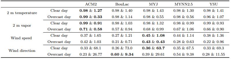
Table 1 shows the correlation coefficient and the root mean square error of the simulated results and the observational results of different schemes. From the table, the simulated results of the 5 schemes are generally good for the 2 m temperature and 2 m vapor. Except for the weak correlation with the vapor under overcast condition (0.57~0.71), the correlation coefficients between the simulations of all the schemes and the observed temperature under both condition are 0.96~0.99, and it is similar with the simulations of all the schemes and the vapor under the clear day condition. Therein ACM2 scheme is superior to other schemes both under the clear and the overcast conditions, for which the minimum correlation coefficient is higher than 0.98 except for the vapor under overcast condition. The other four schemes do not have much obvious differences. However, the deviation of the simulated results of wind speed and wind direction is large. The correlation coefficient is between 0.21 and 0.60, and the difference of each scheme is large. Therein the local schemes behave better than the non-local schemes. In comparison, the MYJ scheme is the best, BouLac scheme is the worst. In general, the simulation of the surface meteorological elements does not need to distinguish between the clear or overcast conditions. If the study focuses on temperature and vapor at 2 m height, the ACM2 scheme should be applied. For analysis of wind direction or wind speed, MYJ scheme is suggested.
|
|
Table 1 The correlation coefficient and root mean square of the meteorological factors with different PBL scheme |
The radiosonde data during the ARM test are used to verify the simulated vertical distribution of the meteorological elements of 5 PBL parameterization schemes. The simulated average vertical profiles of the potential temperature, vapor and wind speed are shown in Figs. 5, 6, 7, respectively, at the point of 14:00 and 02:00 in the simulation.

|
Fig. 5 The comparison of the vertical profiles of potential temperature between the observed and the simulated with different PBL scheme during simulated time (a) Clear day at 14:00; (b) Clear day at 02:00; (c) Overcast day at 14:00; (d) Overcast day at 02:00. |

|
Fig. 6 The comparison of the vertical profiles of the vapor between the observed and the simulated with different PBL scheme during simulated time (a) Clear day at 14:00; (b) Clear day at 02:00; (c) Overcast day at 14:00; (d) Overcast day at 02:00. |

|
Fig. 7 The comparison of the vertical profiles of wind speed between the observed and the simulated with different PBL scheme during simulated time (a) Clear day at 14:00; (b) Clear day at 02:00; (c) Overcast day at 14:00; (d) Overcast day at 02:00. |
Figure 5 shows the simulated results of the potential temperature at 02:00 and 14:00 in clear and overcast days, as well as the observations. Fig. 5a and 5c show the vertical potential temperature profile at 14:00 in clear days and overcast days, respectively. All these 5 schemes successfully simulate unstable stratification where the temperature decreases with height near the ground. For the mixing layer, due to the action of solar radiation, the surface sensible heat flux increases and the turbulent mixing is enhanced. The radiosonde data show that the height of the mixing layer reaches 1100 m. All the simulated results are cooler than the observation. Therein, ACM2 and YSU schemes consider the transport effect of the large eddy and have strong turbulence mixing ability, which makes the simulated mixing layer higher, warmer and closer to the observed values. The simulated result is the worst as the turbulence mixing of BouLac scheme is weaker. Under the overcast condition, the compression of the low cloud tends to inhibit the turbulent mixing, which makes the mixing layer reaches only about 800 m. The simulated results of all these 5 schemes are warmer than the observation. Therein, the ACM2 scheme stands out by using the coefficient fconv to control the ratio of the non-local and local effect. Fig. 5b and 5d show the vertical potential temperature profile at 02:00 in clear days and overcast days. Under the clear day condition, the radiosonde data show that there is a strong inversion layer below 200 m, and the intensity of the inversion reaches 2 K/100 m. All these 5 schemes successfully simulate this inversion layer. Under the overcast conditions, the long-wave radiation from the clouds partially offsets the cooling effect of long-wave radiation from the surface, and forms a weak unstable stratification instead of a strong stable inversion layer. All these 5 schemes successfully simulate the weak stable stratification. Therein the ACM2 scheme uses coefficient fconv to control the ratio of the non-local and local effect in order to be close to the observation. The simulated stability of stratification of the YSU and the BouLac schemes are weaker and the heights are higher than observation, while in the MYJ and the MYNN2.5 schemes, they are stronger and lower.
3.3.2 Vertical profiles of the vaporFigure 6 shows the simulated and the observational profiles of the vapor at 02:00 and 14:00 in clear and overcast days. Fig. 6a and 6c show the vapor profiles of 14:00 under the clear and the overcast condition, respectively. In the mixing layer of the clear day (1100 m), the vapor is strongly mixed so that it is uniformly distributed along the vertical direction, which remains at about 15 g·kg-1. The vapor of the mixing layer in the overcast day (800 m) remained unchanged at about 9 g·kg-1. The profile of the vapor reflects the turbulence mixing in the mixing layer. The ACM2 and YSU schemes simulate the higher mixing layer with lower vapor both in the clear and overcast days. However, BouLac scheme, because of the weak turbulence mixing ability, failed to correctly reflect the height of the mixing layer. For the simulated value of the vapor, compared with the observation, all the schemes are larger. In addition, the profiles of the vapor in the clear and overcast days show that the variations of the vapor with height simulated by the local schemes are more intense than that simulated by the non-local schemes. Since the turbulence mixing of the local scheme is weaker, the vapor is less uniformly mixed in the PBL. Fig. 6b and 6d show the vertical profiles of the vapor at 02:00 in the clear and overcast days, respectively. There is a certain degree of inverse humidity both under the clear and overcast conditions, and the inversion is more intense in the clear days, which is mainly caused by the phase change of a large amount of surface vapor under the radiation effect under the clear day condition. All the five schemes can simulate the inversion under these two conditions, and the ACM2 scheme is the closest to the observed value.
3.3.3 Vertical profiles of the wind speedThe simulated results of the vertical profiles of the wind speed at 02:00, 14:00 under the clear and overcast conditions are compared (Fig. 7). Fig. 7a and 7b show the simulated results of the clear days at 02:00 and 14:00. The deviation of the simulated results of each scheme from observation is large in the clear days, and the maximum deviation can reach 8 m·s-1. It can be seen from Fig. 7a that blow 300 m during the day time, only the MYJ scheme can simulate the characteristic that the wind speed increases with height. Between 300 m and 900 m height, the wind speed does not change with height, except the BouLac scheme, the other four schemes are able to simulate this characteristic well. Above 900 m height, there exists a boundary layer jet near 1050 m, except the MYNN2.5 scheme, the other four schemes can simulate this jet, in which the simulated jet of the BL and MYJ schemes is more consistent with the observational results. It can be seen from Fig. 7b that the maximum wind speed occurs around 200 m at night, and the boundary layer jet is formed. All these 5 schemes are able to simulate the increase of the wind speed with height, but the jet is not simulated in these 5 schemes.
Figure 7c and 7d shows the simulated results of the overcast days at 02:00 and 14:00. The simulated results of each scheme are in good agreement with the observational results. It is seen from Fig. 7c that the wind speed increases slowly between 0 to 150 m height during the day time. In the height of 150~900 m, the wind speed varies between 4 and 6 m·s-1, and starts to decrease at a height of about 1350 m. Except the MYJ scheme, the other 4 schemes can simulate the trend of the wind in PBL, and the MYNN2.5 scheme is the most consistent with the observations. It is shown in Fig. 7d that the wind speed increases with height in the range of 0~800 m at night and reaches the maximum at 700 m. Except the BouLac scheme, other 4 schemes can successfully simulate this process.
In general, the simulated wind speeds of the schemes are consistent with the observed values under the overcast condition. Therein, the MYNN2.5 scheme has the best simulation effect for the day time, and the YSU scheme behaves best for the night time. However, the simulation has more deviation under the clear day condition. Therein, the MYJ scheme is the best for the day time simulation, and the deviation of the ACM2 scheme is the smallest for the night time simulation. The poor simulations in the clear days are mainly caused by the wind speed which is essentially affected by the thermal conditions. These processes are more complex under the clear day conditions, because of the solar radiation effect, the radiation inversion and other processes, which cause the uneven atmospheric stratification. Thus, compared to the overcast days, it is much more difficult to simulate the PBL well under the clear day conditions. In addition, the atmosphere is vertically divided into 28 layers below 2 km in this study. Compared with the observational data, the vertical interval is larger, and it is difficult to clearly simulate finer structures at different heights, such as the boundary layer jet.
4 CONCLUSIONSIn the present study, five PBL parameterization schemes (ACM2, BouLac, MYJ, MYNN2.5, YSU) in the WRF model were used to study the meteorological elements and the PBL structure under the clear and overcast conditions. The observational data of the US ARM test were also adopted for a verification of these 5 schemes. The results show that:
(1) Two non-local schemes (ACM2 and YSU) are superior to local schemes for the lifetime of the cloud, the height of the cloud base, and the cloud thickness.
(2) For the temperature and vapor, the ACM2 scheme, which is able to control the ratio of the local effect and non-local effect, is the best both under the clear and overcast conditions, and the correlation coefficient reaches 0.99. For the wind speed and the wind direction, the local schemes are superior both in the clear and overcast conditions, and the correlation coefficient reaches 0.6.
(3) For the vertical profiles of the temperature and the vapor, the non-local schemes (ACM2 and YSU) are better for the unstable conditions at the day time, both under the clear and overcast conditions. Under the condition of weak stability at night, all these 5 schemes can simulate the stable stratification and the inverse structure of the humidity in the clear days, while the ACM2 scheme is optimal for the weak stable stratification and the inverse structure of the humidity in the overcast days.
(4) For the vertical profile of the wind speed, under the unstable condition at the day time, the MYJ scheme is the best for the simulation of the PBL jet and other structures in the clear days. Except the MYJ scheme, the other schemes can simulate the structure of the PBL in the overcast days, of which the MYNN2.5 scheme is the closest to the observation. While under the weak stable condition at night, the deviation between the ACM2 scheme and the observed value is the smallest under the clear day condition, and the YSU scheme performs best under the overcast condition.
In this paper, the simulation analysis is of great significance for the selection of the parameterization scheme of the PBL in the Shouxian area in Anhui Province, which can be applied in the air quality model. However, a specific analysis is needed for other terrain conditions.
ACKNOWLEDGMENTSThis work was supported by the National Natural Science Foundation of China (91544229); National Key Research and Development Plan (SQ2016ZY01002213); Scientific Research Foundation for Returned Scholars, Ministry of Education of China.
| [] | Bougeault P, Lacarrère P. 1989. Parameterization of orography-induced turbulence in a Mesobeta-Scale Mode. Mon.Wea. Rev. , 117 (8) : 1872-1890. DOI:10.1175/1520-0493(1989)117<1872:POOITI>2.0.CO;2 |
| [] | Fan X H, Chen H B, Xia X G, et al. 2010. Aerosol optical properties from the Atmospheric Radiation Measurement Mobile Facility at Shouxian, China. Journal of Geophysical Research:Atmospheres , 115 (D7) : D00K33. |
| [] | Gibbs J A, Fedorovich E, van Eijk A M J. 2011. Evaluating weather research and forecasting (WRF) model predictions of turbulent flow parameters in a dry convective boundary layer. Journal of Applied Meteorology & Climatology , 50 (12) : 2429-2444. |
| [] | Hong S Y, Noh Y, Dudhia J. 2006. A new vertical diffusion package with an explicit treatment of entrainment processes. Monthly Weather Review , 134 (9) : 2318-2341. DOI:10.1175/MWR3199.1 |
| [] | Hu X M, Nielsen-Gammon J W, Zhang F Q. 2010. Evaluation of three planetary boundary layer schemes in the WRF Model. Journal of Applied Meteorology & Climatology , 49 (9) : 1831-1844. |
| [] | Huang W Y, Shen X Y, Wang W G, et al. 2014. Comparison of the thermal and dynamic structural characteristics in boundary layer with different boundary layer parameterizations. Chinese J. Geophys. , 57 (5) : 1399-1414. DOI:10.6038/cjg20140505 |
| [] | Janjić Z I, et al. 1990. The step-mountain coordinate:Physical package. Monthly Weather Review , 118 (7) : 1429-1443. DOI:10.1175/1520-0493(1990)118<1429:TSMCPP>2.0.CO;2 |
| [] | Kim Y, Sartelet K, Raut J C, et al. 2013. Evaluation of the weather research and forecast/urban model over greater Paris. Boundary-Layer Meteorology , 149 (1) : 105-132. DOI:10.1007/s10546-013-9838-6 |
| [] | Lu Z R. 2014. Study of aerosol optical properties in Shouxian, Anhui based on ARM mobile facility[Master thesis] (in Chinese). Nanjing: Nanjing University of Information Science & Technology. |
| [] | Nakanishi M, Niino H. 2004. An improved Mellor-Yamada level-3 model with condensation physics:Its design and verification. Boundary-Layer Meteorology , 112 (1) : 1-31. DOI:10.1023/B:BOUN.0000020164.04146.98 |
| [] | Pleim J E. 2007. A combined local and nonlocal closure model for the atmospheric boundary Layer.Part Ⅱ:Application and evaluation in a mesoscale meteorological model. Journal of Applied Meteorology & Climatology , 46 (9) : 1396-1409. |
| [] | Qiu G Q, Li H, Zhang Y, et al. 2013. Applicability research of planetary boundary layer parameterization scheme in WRF model over the alpine grassland area. Plateau Meteorology , 32 (1) : 46-55. |
| [] | Shin H H, Hong S Y. 2011. Intercomparison of Planetary boundary-layer parametrizations in the WRF model for a single day from CASES-99. Boundary-Layer Meteorology , 139 (2) : 261-281. DOI:10.1007/s10546-010-9583-z |
| [] | Storer R L, van den Heever S C. 2013. Microphysical processes evident in aerosol forcing of tropical deep convective clouds. Journal of the Atmospheric Sciences , 70 (2) : 430-446. DOI:10.1175/JAS-D-12-076.1 |
| [] | Wang T J, Zhang L, Hu X J, et al. 2013. Numerical simulation of summer boundary layer structure over undulating topography of Loess Plateau simulated by WRF model. Plateau Meteorology , 32 (5) : 1261-1271. |
| [] | Wang Y, Zhang L, Hu J, et al. 2010. Verification of WRF simulation capacity on PBL characteristic and analysis of surface meteorological characteristic over complex terrain. Plateau Meteorology , 29 (6) : 1397-1407. |
| [] | Zhang L. 2012. Verification of WRF simulation capacity for SACOL meteorological elements on different PBL schemes near the ground surface in winter[Master thesis] (in Chinese). Lanzhou: Lanzhou University. |
| [] | Zhang X P, Yin Y. 2013. Evaluation of the four PBL schemes in WRF Model over complex topographic areas. Transactions of Atmospheric Sciences , 36 (1) : 68-76. |