 2017, Vol. 60


2 Key Laboratory of Mineral Resources, Institute of Geology and Geophysics, Chinese Academy of Sciences, Beijing 100029, China;
3 115 Coal Geological Exploration Institute, Shanxi Datong 037003, China
The artificial source CSAMT (Controlled Source Audio-frequency Magneto-Telluric) method is widely used in geological surveys for oil and gas, metal mineral resources, geothermal energy, and in hydro-geological, environmental and coalfield geology explorations (Kaufman and Keller, 1983; An and Di, 2010) owing to its strong signal and high efficiency. Following the MT (Magneto-Telluric) method, the CSAMT method works in the far-zone and defines apparent resistivity by means of the ratio formula.
The MT uses ratio apparent resistivity (Cagniard, 1953) because of its unknown nature source. Ideally, ratio apparent resistivity could cancel the noise interference when electric field and magnetic field suffered the same disturbance from noise. However, in many cases, electric field and magnetic field are disturbed by different interference. Since the transmit current is known, the electric field and magnetic field of CSAMT could be separated from each other for better interpretations.
It is known from WFEM (Wide Field Electro-Magnetic) method (He, 2010) that observation of single component would not reduce information of the earth. Similarly, CSAMT as artificial source method could realize single component observation.
The single component apparent resistivity could be derived through far-zone asymptotic expressions of electromagnetic field of a uniform earth (Chen and Yan, 1995), or through iterative algorithm (Di et al., 2008), or through curve fitting (Routh and Oldenburg, 1999; Li et al., 2000; An et al., 2013; Yin et al., 2014). In this paper, we analyze the disturbance of noise in ratio apparent resistivity of CSAMT, and use single component phase curve fitting inversion to cancel static offset (Maclennan and Li, 2013) and use the number of frequencies as layer number for initial model to enhance the resolution of fitting inversion. The exploration of water-filled goaf in Datong, Shanxi Province shows that the single component prospecting and interpreting method is effective.
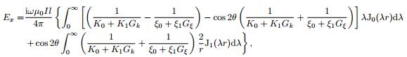
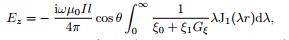
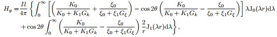
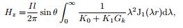
2 RATIO APPARENT RESISTIVITY OF CSAMT 2.1 Ratio Apparent ResistivityGenerally, the source used in CSAMT is grounded electric dipole. In the frequency range (0.1 Hz < f < 105 Hz), the displacement current is far less than the conduction current (Ward and Hohmann, 1992), and the quasistatic expressions of an electric dipole on the earth are (Cao, 1982; Chen and Yan, 1995) :
|
(1a) |

|
(1b) |
|
(1c) |

|
(1d) |
|
(1e) |
|
(1f) |
where, the significance of each parameter and function, and the infinite integral algorithm are explained in Appendix A.
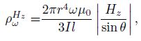
Figure 1 depicts the field distribution on a uniform earth (in agreement with the field distribution on a layered earth) calculated by Eq.(1) when the electric dipole Il = 1, earth resistivity ρ = 50 Ωm, frequency f = 2 kHz, and formation factor Gk = Gξ = 1. The electric field Ex (Fig. 1a) agrees with the magnetic field Hy (Fig. 1e) in the form, and Ey (Fig. 1b) agrees with Hx (Fig. 1d) in the form; thereby, Ex/Hy or Ey/Hx as ratio apparent resistivity is valid. The vertical components, electric field Ez (Fig. 1c) and magnetic field Hz (Fig. 1f) do not agree with each other in forms. Since Ez is difficult to observe, it is not used in the surface exploration usually.

|
Fig. 1 Electromagnetic field distribution on the surface of uniform earth by CSAMT electric dipole
(The position and direction of Il = 1 · |
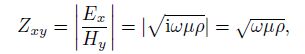
The common scalar observation, such as standard configuration of GDP32 and V8, is six-electric field Ex and one-magnetic field Hy for every array. According to the plane wave impedance formula in good conductor (Feng, 2010)
|
(2) |
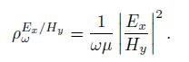
where, μ is earth magnetic permeability, usually μ = μ0 = 4π× 10-7 H·m-1, the permeability of vacuum; ρ is earth conductivity. The ratio apparent resistivity derived from Eq.(2) is (Cagniard, 1953)
|
(3) |
The observation area should be in principal value of the lobe (see Fig. 1) because of the directivity of the CSAMT source. The ratio apparent resistivity of Eq.(3) could, ideally, cancel disturbance and obtain some anti-disturbance capability if electric field Ex and magnetic field Hy suffer the same disturbance and the same distortions. However, there are seldom the cases that the disturbance is ideally canceled to obtain high quality observed data in exploration engineering. More generally, the electric field component or magnetic field component will exhibit different characters under the different interference. Different polarization direction, different environmental and geological conditions (such as poorly grounded electric dipole) will bring different observation quality and different effect on electric field or magnetic field. Thus, the ratio apparent resistivity can not completely cancel noise disturbance in this situation.
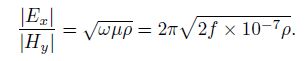
2.2 Analysis of Electromagnetic InterferenceFrom Eq.(2), the plane wave impedance in good conductor, we have
|
(4) |
By Eq.(4), when the earth resistivity and the frequency are lower, the value of 

Within the frequency range of geophysical electromagnetic exploration, the most common source of interference is 50 Hz and its harmonic industry interference. Therefore, special trap circuit is designed in CSAMT instrument. And the random white noise with zero mean could be canceled by continuous stack average. But nonzero mean colored noise (Tang et al., 2012; Jing et al., 2012; Maclennan and Li, 2013) would influence the observed data. Similarly, if noise could not be canceled completely, the noise included in electric and magnetic field components would be different. When earth resistivity and noise frequency are higher, the electric field noise is stronger; and when earth resistivity and noise frequency are lower, the magnetic field noise is stronger.
For example, Fig. 2 is the CSAMT observation data of Line 2 160 of Changqing Oil Field in North Shaanxi. The ratio apparent resistivity ρωEx/Hy in Fig. 2a has obvious distortion. Figs. 2b and 2c are electric field Ex and magnetic field Hy separated from ratio resistivity respectively. The electric field curve is smooth and has no obvious distortion; however, the noise through low resistivity earth to observation point with dominant magnetic field caused Hy disturbance in 0.1~1 Hz frequency range so that the ratio apparent resistivity is deteriorated by magnetic field.

|
Fig. 2 CSAMT observation data of 2 Line 160 station of Changqing Oil Field in North Shaanxi (a) Ratio apparent resistivity curve; (b) Electric field |Ex| curve; (c) Magnetic field |Hy| curve. |
In addition, the ground vibration could disturb magnetic channel signal to result magnetic field data of poor quality. Fig. 3 represents the data of the observation point beside the road (L4 line MON20 array with six-electric field and one-magnetic field of Jiangjiawan Coal Mine in Datong, Shanxi Province), ratio apparent resistivity curves have obvious distortion (Fig. 3a), while six electric field Ex components have no obvious distortion (Fig. 3b), and the noise of Hy at one observation point (Fig. 3c) influence the ratio apparent resistivity at six observation points. Moreover, in Fig. 3b, the smooth fluctuation of electric field Ex in 2~10 kHz, which reflect geology situation, is amplified by ratio apparent resistivity to exhibit distortion in corresponding frequency range similar to that suffered from interference in Fig. 3a. Although according to electromagnetic method exploration rules (SY/T, 2012), observation point should be away from vibration sources, such as the busy highway, drilling platform and so on, it is hard to avoid increasing dense traffic network under the situation of rapid economic development. If using different character of each component under different interference, we not only extend CSAMT exploration area but also find new way to cancel interference.

|
Fig. 3 CSAMT observation data of L4 line MON20 array of Jiangjiawan Coal Mine in Datong, Shanxi Province (a) Ratio apparent resistivity curve; (b) Electric field |Ex| curve; (c) Magnetic field |Hy| curve. |
Each component of electromagnetic field has different behavior of topography and surface electrical heterogeneity (Qiu et al., 2011) and different behavior of different field-zone and record point (Chen and Yan, 2005). Therefore, when observed data is of poor quality, we could separate electric and magnetic field components from CSAMT observed record to mine available data.
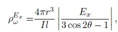
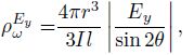
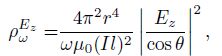
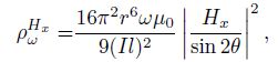
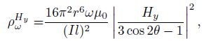
3 INVERSION OF CSAMT SINGLE COMPONENT APPARENT RESISTIVITY 3.1 CSAMT Component Apparent ResistivityApparent resistivity definition and algorithm is an important content of electromagnetic exploration (Li, 2012), and apparent resistivity-depth section is an important map of the exploration results. In MT method, the absolute value of apparent resistivity can not be determined by the single electromagnetic component because of unknown current intensity of the natural source. Because of known and controlled source, the single component resistivity of CSAMT can be determined with formation factor Gk = Gξ = 1 of all-zone Eq.(1) and (Chen and Yan, 1995) :
|
(5a) |
|
(5b) |
|
(5c) |
|
(5d) |
|
(5e) |
|
(5f) |
where, r is the distance between transmitter and receiver.
Owing to limited transmitter power, receiver sensitivity, and signal-noise ratio, it is impossible to do the far-zone observation completely so the relationship between apparent and real earth resistivity is more complex. As shown in Fig. 4a, in far-zone, ρωEx and ρωHy, i.e., the electric and magnetic field apparent resistivity of uniform earth, represent the real resistivity of the earth; however, from middle-zone to near-zone, ρωEx is down to 1/2 of the real value, ρωHy falls along 63°26'. As shown in Eq.(5), between single component apparent resistivity and field intensity or square of field intensity, there is only one coefficient difference and the false extremum problem still exists (Spies and Eggers, 1985; Chen and Yan, 1995; Shi, 1999). By the interference result of electromagnetic wave at formation interfaces, when lower layer resistivity is lower than upper layer resistivity, the apparent resistivity will first rise to a maximum and then fall down; and when lower layer resistivity is higher than upper layer resistivity, the apparent resistivity will first fall to a minimum and then rise up. The false extremum might enlarge the amplitude of apparent resistivity curves to project the middle high resistivity layer of K-type curve, but also might mislead the deduction of layer-electrical property. Thus, as shown in Fig. 4b, the apparent resistivity of A-type section presents a high-low-high shape, the shape of H-type section. The obtained apparent resistivity section will present tripe that does not reflect the real change of earth resistivity. But compared with ratio apparent resistivity, single component apparent resistivity defined in Eq. (5) improves the false extremum slightly.

|
Fig. 4 All-zone apparent resistivity curves (a) The apparent resistivity curves of uniform earth; (b) The minimum of apparent resistivity curves of A-type curves section. |
The maximum and minimum of frequency-domain sounding curves serve as the characteristic points in fitting inversion and the false extrema increase the number of extreme value points or enlarge the amplitude of extreme value in contrast to time-domain TEM (Transient Electro-Magnetic) curve with similar shape of exponential decay. Therefore, the fitting inversion of CSAMT converges fast, commonly, the fitting error of theoretical curves is < 1%, and the fitting error of curves near horizontal strata in good quality is < 5% (Chen and Yan, 1995). In setting initial parameter of fitting inversion, we do as follows:
(1) If apparent resistivity curve shows a far-zone asymptote, take asymptote value as the resistivity of the surface layer, for far-zone apparent resistivity represents the real resistivity of surface layer; if apparent resistivity curve shows a near-zone asymptote, take twice asymptote value as the resistivity of bottom layer, for near-zone apparent resistivity is 1/2 resistivity of bottom layer.
(2) The number of layers decides the fitting inversion result. When assumed number of layers is equal to real number of layers, the fitting results are closest to the real formation. If assumed number of layers is more than real number of layers, the number will return to real number of layers; if assumed number of layers is less than real number of layers, the number will not increase automatically. So it is necessary to assume the number of layers by referring to geological data.
(3) According to the basic theory of modified generalized inverse matrix (Chen et al., 1983; Chen and Yan, 1995), the number of layers could be equal to the number of frequencies at most. In practical exploration, the number of electric layers revealed by electric logging is up to dozens. Taking the number of frequencies as the number of layers could not only let the result of inversion close to real formation as far as possible but also obtain finer resistivity-depth section to express formation resistivity.
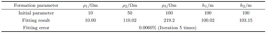
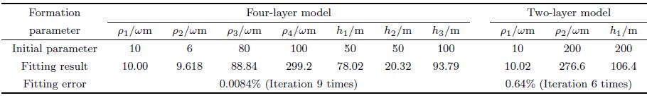
Table 1 and Table 2 are the results of inversion of electric field amplitude curve of A-type geo-electric section in Fig. 4b. The model of three layers produced the best result since the initial number of layers is equal to the real number of layers. But for unknown number of layers, it is necessary to assume more layers for prospecting purpose. In Table 2, although the inversion results with four-layer initial parameter is not as good as the results with three-layer initial parameter, the resistivity of first and second layer is close to that of the first layer; the third layer is equivalent to the second layer of the actual formation, and the fourth layer is equivalent to the third layer of the actual formation; compared with two-layer model, it is closer to the real formation.
|
|
Table 1 Inversion of electric amplitude curve for three layers (Fig. 4b) using a three-layer model |
|
|
Table 2 Inversion of electric amplitude curve for three-layers (Fig. 4b) using four-and two-layer models |
In investigation of inversion algorithms, the dependency on initial parameters is used as a criterion of algorithm effectiveness generally. However, in exploration engineering, geological data should be fully used because introducing geological or other geophysical data as constraint is the indispensable procedure and guarantee of success for practice problems (Hohmann and Raiche, 1992), as well as requirement of exploration technical specification (SY/T, 2012) and the way to exploit geological data.
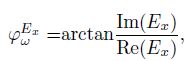
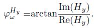
4 CSAMT SINGLE COMPONENT PHASEApparent phase (abbreviated as phase) is another basic parameter in CSAMT interpretation. Since it is difficult to observe, phase was seldom used in the past. With the development of electronic technology, many instruments have the function of observing the phase. Apparent phase also has ratio or single component definition. Ratio apparent phase is the phase difference between electric field phase and magnetic field Hy phase, and single component apparent phase is the ratio of imaginary part to real part of single component field (Chen and Yan, 1995; Li, 2012). For example:
|
(6a) |
|
(6b) |
By Cauchy formula (Kaufman and Keller, 1983) or Hilbert transform (Vanyan et al., 1961), the relationship between single component field amplitude and phase is
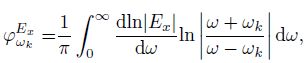
|
(7a) |
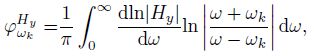
|
(7b) |
where, ωk is circular frequency; ψωkEx and ψωkHy are phase at frequency k, equal to the integral of logarithmic amplitude gradient in the whole frequency domain, which are determined by the slope of field amplitude curve at the dual logarithm coordinate, consequently phase is not affected by static effect and has no offset. Fig. 5 is the responses of field amplitude and phase in CSAMT exploration for Yanzishan Coal Mine, Datong, Shanxi Province where exists surface electrical heterogeneity. The electric field amplitude curves of L15-400 and L15-520 have up-and downward translation relative to L15-280 (Fig. 5a) while magnetic field amplitude curves have no such a translation because of no surface magnetic heterogeneity (Fig. 5b); both electric field phase (Fig. 5c) and magnetic field phase (Fig. 5d) have no translation except the changes with formation resistivity. In most cases, earth is non magnetic, magnetic field is not affected by static offset. Since magnetic field Hy observation point is sparse in scalar observation (Six-electric field and one-magnetic field for each array) and is less sensitive to formation resistivity (comparison of Figs. 5a and 5b), using electric field phase is a way to avoid static offset. If the instrument has no such a function of observing phase or observed data is of poor quality, phase could be calculated from field amplitude by Eq.(7), which is equivalent to the procedure by Vanyan et al. (1961) and Kou and Zhou (1988) through complex resistivity ρω = |ρω|eiψω to obtain phase.

|
Fig. 5 Response of static offset along L15 Line in CSAMT exploration for Yanzishan Coal Mine 315 Mining Area in Datong Coal Field, Shanxi Province (a) |Ex| curves of observation point 280, 400, 520; (b) |Hy| curves of observation point 400 and 520; (c) ψωkEx curves of observation point 280, 400 and 520; (d) ψωkHy curves of observation point 400 and 520. |
The extreme point of phase curve corresponds to inflexion of amplitude curve, which is useful to deduce the type of geo-electrical section (comparison of Figs. 5a and 5c, 5b and 5d). In quantitative interpretation, phase response and amplitude response have equal effect, phase could not provide more information (Kaufman and Keller, 1983), but could provide correct interpretation when surface electrical heterogeneity exists.
In CSAMT exploration of water-filled goaf of 2#, 4# and 14# in 315 Mining Area of Yanzishan Coal Mine in Datong, the maximum detection depth from the burial depth of coal seam is 350 m, the distance between transmitter and receiver according to far-zone condition and ratio of signal to noise is 3000~3500 m. The point space is 20 m, frequency range is 10.6735008533 Hz and the total frequencies are 31. Observed electric field curves exhibit the translation by surface electrical heterogeneity for there are loess, mildlay, Loam, sand, scree and gravel inter-distributed on the surface of the observation area, as shown in Fig. 5, while general inverse matrix inversion to determine thickness and subdivision could be used for the landform is flat and formation is stable in the area. Table 3 is the average resistivity and thickness as initial parameters for inversion.
|
|
Table 3 Average resistivity and bed thickness of 315 Mining area of Yanzishan Coal Mine in Datong Coal Field, Shanxi Province |
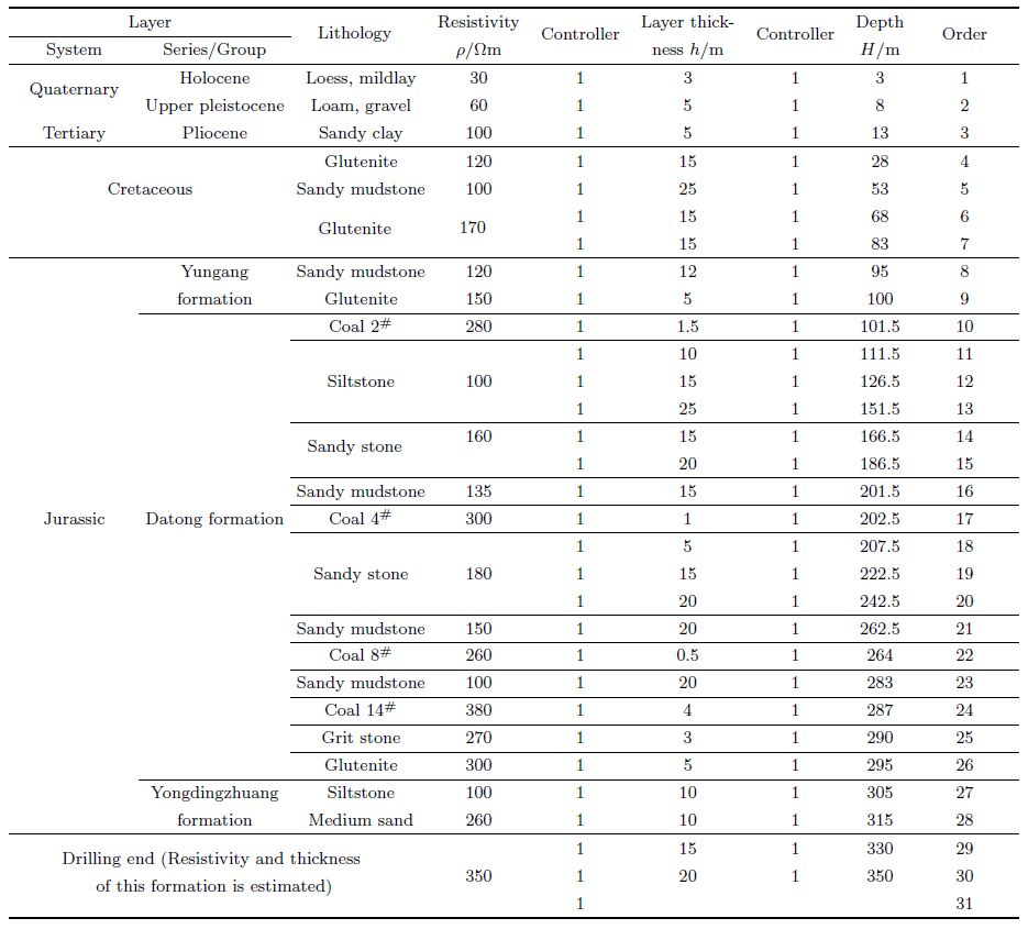
Figure 6a shows the resistivity-depth section of fitting inversion of electric field amplitude curves of L15, and around L15-400 and L15-520 point there are a resistive string of beads caused by up and down translation of curves. Usually, translation of curves does not represent vertical electrical variation in deep formation, conversely drill, geology and mining data indicate there seem no graben developed, no fault more than 5 m and the revealed collapse column ends at coal 14#. For this, in fitting inversion we use electric field phase curves, and the obtained resistivity-depth section is shown in Fig. 6b. The result of phase inversion shows clear layered formation in agreement with general structure of the area. According to geological and mining data, the low resistivity thin layer at the depth of 100 m is deduced as water-filled goaf of coal 2#, L15-360~L15-560 is water-rich zone, L15-500~L15-540 is strong water-rich zone; at the depth of 200 m, the coal 4# occurred, low resistivity has not been seen, thus water-filled deduction is not done; the secondary high resistivity in L15-225~L15-250 is deducted as unworkable coal 8#; high resistivity zone at the depth of 275~325 m is no mined or mined but no water-filled coal 14#. After completion of exploration, the water yield of dewatering drill at point L15-520 affirms deduction of coal 2# and coal 14# filled with water at this segment.

|
Fig. 6 Resistivity-depth section along L15 Line in CSAMT exploration for Yanzishan Coal Mine 315 Mining Area in Datong Coal Field, Shanxi Province (a) Fitting inversion of electric field amplitude curves (Iteration 10 times, fit error: points 400 and 520 are 6.72% and 9.17%, and other points are 2.93%~4.26%); (b) Fitting inversion of electric field phase curves (Iteration 10 times, fit error: 2.68%~3.98%). |
Electric field and magnetic field have different sensitivity to interference, therefore electric and magnetic field component could be separated from ratio apparent resistivity to cope with different interference environment. When formation is stable and the dip angle is not more than 5°, quantitative inversion is the way to obtain real formation resistivity. The far-zone and near-zone asymptote of apparent resistivity could present relatively accurate surface resistivity and rough bottom layer resistivity for initial parameters of inversion. Setting the layer number near to the real layer number in fitting inversion produces finer resistivity-depth section. Furthermore, inversion of observed (or transformed) phase curves could cancel static offset without additional error. The CSAMT exploration of water-filled goaf in Yanzishan Coal Mine, Shanxi Province verified the effectiveness of single component exploration and interpretation.
Complexity of geological problems need to seek the solution from more angles in more ways. While the single component of CSAMT enriched the means of detection, ratio apparent resistivity also cannot be ignored. For example, sometimes the effective value of distorted transmitter waveform will be not accurate at high frequencies, the ratio apparent resistivity independent of current performs better at high frequencies.
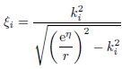
Appendix A The Significance of Each Parameter and Function in Eq.(1) and Digital Filter AlgorithmIn Eq.(1), i stands for the imaginary part of a complex number, I is transmitting current, l is the length of a dipole, ω = 2πf is circular frequency, f is frequency, μ is the magnetic permeability of a non-magnetic earth and takes the permeability of vacuum μ0 = 4π × 10-7, θ is the angle between the point and the source point, as shown in Appendix Figure (In exploration, AB usually stands for the dipole l, the electric component is obtained by measuring the voltage between two ends of grounded wire MN and then Ex = VMN/MN), J0 (λr) and J1 (λr) are first kind 0 order and 1 order Bessel function respectively, where, λ is the component of the wave vector pointing from source to the field point, r is the distance from source point to field point, Gk and Gξ are formation factors. The recursion formulas from the mth-layer upward are
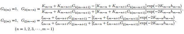
|

|
Fig. Appendix Fig Scalar CSAMT configuration plan |
where 
Digital filter algorithm takes single component electric Ex as an example. Make variable substitution
|
Eq.(1a) is changed to
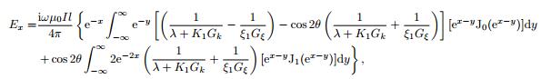
|
rewrite it as digital filter form
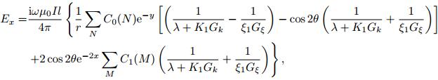
|
where, C0 (N) and C1 (M) correspond to filter coefficients of 0 order and 1 order Bessel function, N and M are the number of the filter coefficients. This paper used the filter coefficients N = 51 (Verma and Koefoed, 1973) and the filter coefficients M = 47 (Koefoed et al., 1972) and the coefficients η = x-y. For canceling the end effect and accelerating convergence, it is necessary to minus the term of a uniform half space from the sum of filter coefficients and then plus the close expression of a uniform half space (Chen and Yan, 1995). After arrangement, we have
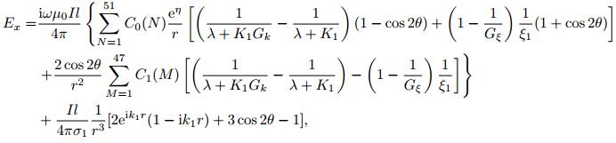
|
where, 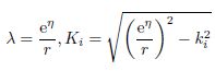
This work was supported by the National Natural Science Foundation of China (41374129, 41474095), Science and Technology Project of Shanxi Province (20100321066).
| [] | An Z G, Di Q Y. 2010. Application of the CSAMT method for exploring deep coal mines in Fujian Province, Southeastern China. Journal of Environmental and Engineering Geophysics , 15 (4) : 243-249. DOI:10.2113/JEEG15.4.243 |
| [] | An Z G, Di Q Y, Wang R, et al. 2013. Multi-geophysical investigation of geological structures in a pre-selected high-level radioactive waste disposal area in Northwestern China. Journal of Environmental and Engineering Geophysics , 18 (2) : 137-146. DOI:10.2113/JEEG18.2.137 |
| [] | Cagniard L. 1953. Basic theory of the magneto-telluric method of geophysical prospecting. Geophysics , 18 (3) : 605-645. DOI:10.1190/1.1437915 |
| [] | Cao C Q. 1982. The low-frequency characteristics and the problem of penetration of high resistance shielding layer for horizontal electric dipole parametric depth sounding. Chinese J. Geophys. (in Chinese) , 25 (6) : 516-537. |
| [] | Chen M S, Chen L S, Wang T S, et al. 1983. The interpretation of magnetotelluric and electrical sounding's data by modified generalized inverse matrix. Chinese J. Geophys. (Acta Geophysica Sinica) (in Chinese) , 26 (4) : 390-400. |
| [] | Chen M S, Yan S. 1995. On Problems in Frequency Electromagnetic Soundings (in Chinese)[M]. Beijing: Geological Publishing House: 69 -72. |
| [] | Chen M S, Yan S. 2005. Analytical study on field zones, record rules, shadow and source overprint effects in CSAMT exploration. Chinese J. Geophys. (in Chinese) , 48 (4) : 951-958. |
| [] | Di Q Y, Wang R, et al. 2008. Controlled Source Audio-Frequency Magneto Tellurics (in Chinese)[M]. Beijing: Science Press . |
| [] | Feng E X. 2010. Electromagnetic Field and Electromagnetic Wave[M]. Xi'an: Xi'an Jiaotong University Press . |
| [] | He J S. 2010. Wide Field Electromagnetic Method and Electrical Method with Pseudo-Random Signal (in Chinese)[M]. Beijing: Higher Education Press . |
| [] | Hohmann G W, Raiche A P. 1992. Inversion of CSAMT Data (in Chinese). //Nabighian M N ed. Electromagnetic Method in Applied Geophysics Volume 1, Theory. Zhao J X, Wang Y J Trans. Revised by Chen Y S. Beijing: Geological Publishing House, 461. |
| [] | Jing J E, Wei W B, Chen H Y, et al. 2012. Magnetotelluric sounding data processing based on generalized S transformation. Chinese J. Geophys. (in Chinese) , 55 (12) : 4015-4022. DOI:10.6038/j.issn.0001-5733.2012.12.013 |
| [] | Kaufman A A, Keller G V. 1983. Frequency and Transient Soundings[M]. New York: Elsevier Science Publishing Company Inc . |
| [] | Koefoed O, Ghoch D P, Polmen G J. 1972. Computation of type curves for electromagnetic depth sounding with a horizontal transmitting coil by means of a digital linear filter. Geophysical Prospecting , 20 (2) : 406-420. DOI:10.1111/gpr.1972.20.issue-2 |
| [] | Kou S W, Zhou J G. 1988. The phase transformation method in electromagnetic frequency sounding. Geophysical & Geochemical Exploration (in Chinese) , 12 (6) : 433-443. |
| [] | Li X B, Oskooi B, Pedersen L B. 2000. Inversion of controlled-source tensor magnetotelluric data for a layered earth with azimuthal anisotropy. Geophysics , 65 (2) : 452-464. DOI:10.1190/1.1444739 |
| [] | Li Y M. 2012. Frequency Sounding Method and the Chart of Frequency Sounding Generated by a Electric Dipole Source (in Chinese)[M]. Xuzhou: China University of Mining and Technology Press . |
| [] | Maclennan K, Li Y G. 2013. Denoising multicomponent CSEM data with equivalent source processing techniques. Geophysics , 78 (3) : E125-E135. DOI:10.1190/geo2012-0226.1 |
| [] | Qiu W Z, Yan S, Xue G Q, et al. 2011. Action of CSAMT field components in mountainous fine prospecting. Progress in Geophysics (in Chinese) , 26 (2) : 664-668. |
| [] | Routh P S, Oldenburg D W. 1999. Inversion of controlled source audio-frequency magnetotellurics data for a horizontally layered earth. Geophysics , 64 (6) : 1689-1697. DOI:10.1190/1.1444673 |
| [] | Shi K F. 1999. Controlled Source Audio-Frequency Magnetotelluric Theory and Application (in Chinese)[M]. Beijing: Science Press . |
| [] | Spies B R, Eggers D E. 1986. The use and misuse of apparent resistivity in electromagnetic methods. Geophysics , 51 (7) : 1462-1471. DOI:10.1190/1.1442194 |
| [] | SY/T 5772-2012. 2012. China Petroleum Standardization Committee. Technical rules of controlled source audio magnetotelluric exploration. 2012-08-23 issue, 2012-12-01 put into effect. |
| [] | Tang J T, Xu Z M, Xiao X, et al. 2012. Effect rules of strong noise on magnetotelluric (MT) sounding in the Luzong ore cluster area. Chinese J. Geophys. (in Chinese) , 55 (12) : 4147-4159. DOI:10.6038/j.issn.0001-5733.2012.12.027 |
| [] | Vanyan L L, Kaufman A A, Terekhin E I. 1961. Computation of phase curves for frequency sounding by transform means. Prikl. Geofiz. , No. 30. |
| [] | Verma R K, Koefoed O. 1973. A note on the linear filter method of computing electromagnetic sounding curves. Geophysical Prospecting , 21 (1) : 70-76. DOI:10.1111/gpr.1973.21.issue-1 |
| [] | Ward S H, Hohmann G W. 1992. Electromagnetic Theory for Geophysical Applications (in Chinese). //Nabighian M N ed. Electromagnetic Method in Applied Geophysics Volume 1, Theory. Zhao J X, Wang Y J Trans. Revised by Chen Y S. Beijing: Geological Publishing House, 125. |
| [] | Yin C C, Qi Y F, Liu Y H, et al. 2014. Trans-dimensional Bayesian inversion of frequency-domain airborne EM data. Chinese J. Geophys. (in Chinese) , 57 (9) : 2971-2980. DOI:10.6038/cjg20140922 |