 2017, Vol. 60


Seismic anisotropy is closely related to the mineral composition, temperature and pressure conditions, stress state and strain history of the Earth's material. It has become a useful tool for detecting the interior deformation of the Earth (Babuska and Cara, 1991; Rabbel and Mooney, 1996). Earlier studies suggest that seismic anisotropy exists mainly in the upper mantle, or more precisely the uppermost mantle, and is caused by the lattice-preferred orientation of olivine, which is driven by the plastic flow of mantle materials under hightemperature and high-pressure environment (Nicolas and Christensen, 1987; Savage, 1999). As a convenient and efficient method, SKS splitting analysis is widely used in various studies of upper mantle anisotropy (Vinnik et al., 1989; Silver and Chan, 1991).
Recent evidence shows that the splitting delay of Moho Ps conversion can reach to 0.2~0.7 seconds beneath the Chugoku district in Japan (Nagaya et al., 2008), suggesting that crustal anisotropy may affect the interpretations of SKS splitting in certain regions. The study of theoretical seismograms also proves that SKS wave will split when the average shear-wave anisotropy of the crust is higher than 1% (Yao et al., 2016). Therefore, crustal anisotropy study is not only crucial for understanding the mechanism of crustal deformation, but also the prerequisite for the interpretation of upper mantle anisotropy.
The origin of crustal anisotropy may be distinct at different depth. The alignment of cracks and microcracks has been considered as the main cause of stress-induced anisotropy in the upper crust (Crampin, 1987). While the preferred orientation of minerals contributes mostly to seismic anisotropy in the middle and lower crust, and is related to the ductile deformation or plastic flow of crustal materials (Weiss et al., 1999; Savage, 1999). In general, crustal anisotropy possesses stratified property. Therefore, any analysis based on single-layered crustal model can only provide rough estimates of crustal anisotropy. Since Receiver Function (RF, refers to P receiver function) is sensitive to seismic velocity discontinuities within the crust, the RF method has advantages in mapping the stratification of crustal anisotropy and has become a hotspot in the seismic anisotropy studies (Fang and Wu, 2009).
Yao (1989) is the earliest one in China to study crack-induced anisotropy from teleseismic Ps conversions. McNamara and Owens (1993) extended the shear-wave splitting method to RF data by using Moho Ps phases. According to the knowledge from synthetic seismograms, Levin and Park (1997) confirmed that crustal anisotropy with tilted symmetry axis could produce similar wavefield pattern as that from dipping Moho. Following this idea, Okaya and McEvilly (2003) studied the variations of wavefield pattern with respect to the plunge of anisotropic symmetry axis, while Savage (1998), Frederiksen and Bostock (2000) and Xu et al. (2006) focused on the differences of RF wavefield between dipping interface and crustal anisotropy.
The backazimuthal pattern generated by arbitrary transverse isotropic (ATI) models has been intensively studied (Frederiksen and Bostock, 2000; Tian et al., 2008). Nagaya et al. (2008) went further to investigate RF wavefield pattern from two-layered ATI model. The results from real data experiments demonstrate that horizontal transverse isotropic (HTI) models are not appropriate for the studies of highly deformed crust (Xu et al., 2006; Qi et al., 2009). In such cases, ATI models have to be considered. In addition, relatively complex models (such as multi-layered anisotropy, anisotropic sedimentary layer, transition layer that consists of thin anisotropic layers) should get attentions as well.
Nevertheless, the theoretical study of RF wavefield has provided a basis for extracting depth-dependent anisotropic parameters by RF waveform inversion. Studies of multi-layered crustal anisotropy based on waveform inversion have already obtained a number of meaningful results in several regions (Ozacar and Zandt, 2004; Sherrington et al., 2004; Tian et al., 2008). This method suits specifically to the stratified ATI media, and is superior to shear-wave splitting analysis. Recently, new methods without waveform modeling have been proposed (Liu and Niu, 2012; Rümpker et al., 2014; Schulte-Pelkum and Mahan, 2014). Those methods exploit some but not all features of the backazimuthal pattern in RF wavefield, and therefore have limitations in application.
The real RF data usually contain interference signals from laterally heterogeneous media, especially the transverse component which is sensitive to lateral scattering (Qi et al., 2016). Besides, the reverberations from the sedimentary structure can also reduce the SNR of the Ps phases from deep interfaces. These noises significantly increase the difficulty in extracting anisotropic parameters. Also it is worth noting that seismic anisotropy shows strong dependency on the backazimuthal coverage of the data. Due to the geographic location of stations and the distribution of events, the observed RF wavefield is always discrete in backazimuth. In some cases, data are missing in a wide range of backazimuths. The incomplete coverage of data may make the uncertainty increase in the analysis of seismic anisotropy (Girardin and Farra, 1998; Liu and Niu, 2012; Rümpker et al., 2014).
In this paper, we go further to investigate the RF wavefield pattern from stratified crustal anisotropic models, including anisotropic sedimentary layer and transition layer. We introduce a denoising method, based on curvelet transform and compressive sensing, to the noise suppression and wavefield reconstruction of the RF wavefield (Qi et al., 2016). In addition, we assess the capability of extracting depth-dependent anisotropic parameters through waveform inversion of both numerical and observed RF data. We recover the stratification of crustal anisotropy beneath an IRIS permanent station (CTAO) on the east coast of Australia and show agreement with previous results.
2 RF WAVEFIELD FROM STRATIFIED ANISOTROPIC MODEL 2.1 Crustal Anisotropic ModelThe fast-axis and slow-axis ATI models showed in Fig. 1 are two types of anisotropic model. According to Levin and Park (1997), the phase-velocity surface of fast-axis anisotropy is prolate ellipsoid that resembles watermelon, and the phase-velocity surface of slow-axis anisotropy is oblate ellipsoid that resembles pumpkin. In the upper crust, the alignment of cracks and microcracks leads to slow-axis anisotropy. In the middle and lower crust, some of the crustal minerals develop the preferred orientation in the direction of fast axis, while others manifest slow-axis anisotropy (Leidig and Zandt, 2003). Evidences from mineralogical studies suggest that the foliated mica-rich fabric may be the main cause of crustal anisotropy in the middle and lower crust (Weiss et al., 1999; Lloyd et al., 2009). The foliation that formed by crystallographically preferred orientation of mica, usually leads to slow-axis anisotropy (Ward et al., 2012). Although some previous studies use fast axis to model deep crustal anisotropy (Sherrington et al., 2004; Tian et al., 2008), there are more results show that slow-axis anisotropy can produce smaller data fitting residual (Leidig and Zandt, 2003; Ozacar and Zandt, 2004; Zandt et al., 2004; Porter et al., 2011; Audet, 2015). Therefore, we will use slow-axis anisotropy to model the entire depth of crustal anisotropy.

|
Fig. 1 Anisotropic models with tilted axis of symmetry (modified from Leidig and Zandt, 2003) (a) Slow-axis anisotropy; (b) Fast-axis anisotropy. The lightgrey thin ellipse represents the isotropic plane. The angle of the symmetry axis with the vertical direction is the plunge of the symmetry axis. |
For the forward modelling, we develop Matlab codes based on the generalized reflection and transmission coefficients method (Chen, 1993). It does not differ from Levin and Park (1997) in an essential manner. The only difference is that we adopt the analytical expression of ATI elastic tensor derived by Yao and Cai (2009), which improves the calculation accuracy in some degree.
Under the assumption of weak anisotropy (Backus, 1965; Park and Yu, 1992), anisotropic elastic tensor can be approximately divided into the isotropic proportion (characterized by P and S velocity, density) and the anisotropic perturbation (characterized by trend and plunge of anisotropic symmetry axis, magnitude of anisotropy). Such parameterized method is convenient for anisotropic modelling and reduces the degree of freedom for the follow-up data inversion (Levin and Park, 1997).
2.3 RF Wavefield from Fast-axis and Slow-axis AnisotropyFigure 2 shows the synthetic RF wavefield from a single-layered crustal model with both fast-axis and slow-axis anisotropy. The horizontal slowness is 0.0618 s·km-1, which is roughly equivalent to the epicenter distance of 60°. The parameters of the crustal model are given in Table 1. M1 is the model for fast-axis anisotropy (positive magnitude), while M2 is the model for slow-axis anisotropy (negative magnitude). Except for the trend of anisotropy (0° for fast-axis, 180° for slow-axis), the parameters of M1 and M2 are the same.

|
Fig. 2 RF wavefield from the fast-axis and slow-axis anisotropic models (a) Fast-axis: R-component; (b) Fast-axis: T-component; (c) Slow-axis: R-component; (d) Slow-axis: T-component; Red color denotes positive amplitude, blue color negative amplitude. All symbols and colors have the same meaning in the following figures. |
|
|
Table 1 Fast-axis and slow-axis anisotropic model |
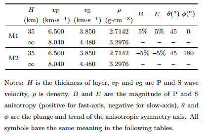
In comparison of Fig. 2(a, b) and Fig. 2(c, d), we can see that the Ps conversions and their multiples possess the same backazimuthal periodicity (360°) in both amplitude and timing. The backazimuths of 0° and 180° are the symmetry directions in the radial component and the anti-symmetry directions in the transverse component. However, the features of the backazimuthal patterns from fast-axis and slow-axis anisotropy are different, and more obviously, the multiples show opposite polarity in the transverse component. These differences can be used to determine the type of anisotropic symmetry axis. Note that the angle difference of 180° in the trend of fast-axis and slow-axis anisotropy is equivalent to the complementary angles of the plunge (Levin and Park, 1997; Erickson, 2002).
2.4 RF Wavefield from Multi-layered Anisotropic ModelRF is the impulse response of the Earth's structure near the receiver. The transmission and reflection waves from each interface involve all layers of anisotropy if there are more than one anisotropic layers in the crust. It is important to know whether we can correctly recover the anisotropic parameters for each layer from complex stratification of anisotropy. Furthermore, the crust usually undergoes movement and deformation in tectonic active areas where low-velocity zones are often detected within the crust (e.g. Tibetan Plateau and North China region). Controlled by the stress and the strain, the low-velocity zones may become the channel for the crustal flow (Beaumont et al., 2001; Liu et al., 2007, 2014), exhibiting observable seismic anisotropy. In addition, Liu and Shao (1985) has already demonstrated that the thin-layer reverberation can enhance the energy of the corresponding converted phases. If the thin layers are anisotropic, whether can they mislead the extraction of anisotropic parameters also requires further studies. Therefore, we will focus on complex anisotropic models in this paper. We calculate the synthetic RF wavefield for several typical models and investigate the impact of anisotropic parameters in each layer on the wavefield pattern.
Here, we consider the case of a two-layer anisotropic model. The parameters of the crustal models are given in Table 2. Model M3 contains two anisotropic layers and one isotropic half-space. The two anisotropic layers have the same anisotropic parameters. Fig. 3 shows the RF wavefield for M3. Between Fig. 3 and Fig. 2(c, d), we find that: (1) the two-layer model can be easily identified through the extra phase Ps1 and its multiples (PpPs1 and PsPs1+PpSs1) in Fig. 3. (2) The P wave projection in the transverse component shows the same polarity in both figures. (3) The backazimuthal patterns of Ps1 in both radial and transverse components are approximately isotropic, while the multiples of Ps1 shows clear anisotropic pattern. (4) The Ps conversion and its multiples from the lowermost interface in both figures have no significant difference. These observations suggest that without considering the multiples, the backazimuthal pattern of the two-layer model with same anisotropic parameters is close to that of the single-layer anisotropy.

|
Fig. 3 RF wavefield from a two-layer anisotropic model: Same anisotropic parameters (a) R-component; (b) T-component. |
|
|
Table 2 Two-layer anisotropic model |
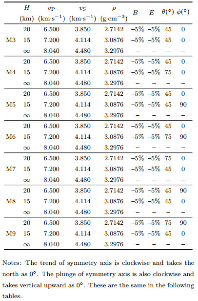
We now consider two-layer models with different anisotropic parameters (upper and lower). In model M4-M6, we fix the anisotropic parameters in the upper layer and only change those in the lower layer. Fig. 4 shows the RF wavefield from these models. In model M4, only the plunge of symmetry axis is modified compared to M3. As showed in Fig. 4(a, b), the corresponding RF wavefield retains the same periodicity as Fig. 3, but the backazimuthal variation of all phases is much more significant. The anisotropic pattern is enhanced when two anisotropic layers have different angles in the plunge of symmetry axis. In model M5, only the trend of symmetry axis is modified, and the angles in both layers are orthogonal to each other. From Fig. 4(c, d), we find that: (1) in the transverse component, the pattern of the P wave projection does not change with the trend in the lower layer (showed by the orange arrows in Fig. 4d). (2) The pattern of the Ps1 multiples (PpPs1 and PsPs1+PpSs1) in the radial component also remains unchanged, regardless of the angle change of both plunge and trend in the lower layer. (3) The change of the trend has more significant impact on Ps2 than that of plunge, since the change of the trend causes 90° shifting of the symmetry or anti-symmetry of Ps2 (showed by green arrows in Fig. 4d). (4) The backazimuthal variation of the Ps2 multiples (PpPs2 and PsPs2+PpSs2) has been weakened significantly in both radial and transverse components. Observations above suggest that the RF pattern is more sensitive to the trend of anisotropic symmetry axis, since the pattern is subject to translation in backazimuth. In the extreme case, when the angles of the trend in two layers are orthogonal to each other, the anisotropic pattern of the multiples from the lower interface can be greatly weakened.

|
Fig. 4 RF wavefield from a two-layer anisotropic model: Lower parameters modified (a) M4, R-component; (b) M4, T-component; (c) M5, R-component; (d) M5, T-component; (e) M6, R-component; (f) M6, T-component. |
Figure 4(e, f) shows the RF wavefield from model M6, in which not only the angles of the trend are orthogonal, but also the angles of the plunge are different. Compared with Fig. 4(c, d) from M5, we find that the backazimuthal pattern only shows some minor changes in energy. Same scenario occurs when comparing the RF wavefield from M3 and M4. It suggests that the backazimuthal pattern of the RF wavefield is less sensitive to the plunge of symmetry axis. Nevertheless, the change of the plunge does cause some energy redistribution along the backazimuth.
In model M7-M9, we fix the parameters in the lower layer and only modify those in the upper layer. The corresponding RF wavefield is showed in Fig. 5. Comparison of Fig. 4 and Fig. 5 shows that: (1) for the two-layer anisotropic model, the parameter changes in the upper and lower layer can cause similar effect to the RF wavefield. More importantly, the RF pattern is more sensitive to the trend of symmetry axis than the plunge in both scenarios. (2) Although the wavefield patterns are quite different between Fig. 4 and Fig. 5, there are some common rules to follow. For example, phases that are generated in either layer are more sensitive to the parameters in that layer. The orange arrows in Fig. 5 show that the angle change of the trend in upper layer causes 90° shifting of the symmetry or anti-symmetry of the P wave projection, while the locations of the green arrows remain the same as those in Fig. 3. (3) The transverse component is more sensitive to the change of anisotropic parameters than the radial component.

|
Fig. 5 RF wavefield from a two-layer anisotropic model: Upper parameters modified (a) M7, R-component; (b) M7, T-component; (c) M8, R-component; (d) M8, T-component; (e) M9, R-component; (f) M9, T-component. |
Models including low-velocity thin layer, sedimentary layer and transition layers of Moho are given in Table 3. In model M10, an anisotropic lowvelocity thin layer is placed in the middle crust, along with isotropic upper and lower layers. As showed in Fig. 6(a, b), the Ps1 (note that Ps1 is the combination of two phases from the upper and lower interfaces of the thin layer) exhibits strong anisotropic pattern, but the anisotropic pattern of the multiples (PpPs1 and PsPs1+PpSs1) is very weak. In addition, the Ps2 from the Moho shows none notable interference by the thin layer above. It seems that the thin anisotropic layer only makes localized impact on its direct converted phase. Note also that, the thin anisotropic layer causes the separation of Ps1 near the backazimuth of 180° in the radial component, which is quite different from the isotropic case (Liu and Shao, 1985).

|
Fig. 6 RF wavefield from anisotropic model with low-velocity thin layer (a) M10, R-component; (b) M10, T-component; (c) M11, R-component; (d) M11, T-component; (e) M12, R-component; (f) M12, T-component. |
|
|
Table 3 Multi-layered anisotropic model |
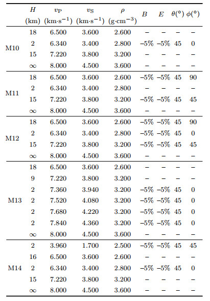
In model M11, an isotropic low-velocity thin layer is sandwiched between anisotropic upper and lower layers. In model M12, the upper and lower layers as well as the thin layer are all anisotropic. The RF wavefield from M11 and M12 are given in Fig. 6(c, d) and (e, f), respectively. The backazimuthal patterns from both models seem quite similar, but still have minor differences in amplitude and timing. It means that, in order to determine whether the thin layer is anisotropic or not, detailed investigation of the RF wavefield with complete backazimuthal coverage is required. This also reminds us that, with the limited data from limited backazimuths, we can only obtain rough estimates of crustal anisotropy.
In model M13, the Moho is replaced by four anisotropic transition layers (total thickness is 8 km), and the layers above the transition layers are isotropic. The corresponding RF wavefield is showed in Fig. 7(a, b). The separation of the converted phases (showed by black arrows) is found near the backazimuth of 180°. Due to the increased number of reflection, the multiples from the top and bottom of the transition layers have separated completely with each other in the radial component, yet no notable anisotropic pattern is observed. From Fig. 6(a, b) and Fig. 7(a, b), we find that the thin anisotropic layer and transition layers only make localized impact on the direct converted phases, while the anisotropic pattern of the multiples is very weak, which is quite different from the thick anisotropic layer. To determine whether the anisotropic signal comes from a thick layer or a thin layer requires the consideration of the multiples and data with complete backazimuthal coverage.

|
Fig. 7 RF wavefield from anisotropic model with transition layers and sedimentary layer (a) M13, R-component; (b) M13, T-component; (c) M14, R-component; (d) M14, T-component. |
Model M14 is modified based on M10 by adding a 2 km anisotropic sedimentary layer at the top. The corresponding RF wavefield is showed in Fig. 7(c, d). Although, the thin sedimentary layer causes significant energy in both radial and transverse components, the anisotropic patterns from the sedimentary layer and the low-velocity thin layer can still be distinguished through the anti-symmetrical feature of the Ps phase in the transverse component.
3 PARTICLE SWARM INVERSIONIn this section, we assess the capability of extracting depth-dependent anisotropic parameters through waveform inversion technique. As mentioned above, the waveform inversion is a common method for studying seismic anisotropy using RF data. In the previous studies, global inversion methods such as genetic algorithm, neighborhood algorithm and simulated annealing are frequently used to prevent the solution from falling into the local minimum (Ozacar and Zandt, 2004; Sherrington et al., 2004; Tian et al., 2008). Different from the S velocity study, the study of seismic anisotropy requires joint inversion of multiple backazimuthal RF traces from both radial and transverse components. Therefore, the efficiency of the method is very important, especially when dealing with a large number of stations.
Recently, a global method called particle swarm optimization (PSO) is proposed and gradually improved (Eberhart and Kennedy, 1995; Shi and Eberhart, 1998; Clerc and Kennedy, 2002). This method is based on the study of the swarm intelligence that the bird flock and fish stock exhibit during their foraging for food. The PSO provides many advantages, including implementation simplicity, friendly parallelization, fast convergence and less parameters to adjust (Eberhart and Shi, 1998; Hassan et al., 2005). And it has been receiving more and more attentions in various research fields (Shaw and Srivastava, 2007; Martnez et al., 2010; Shi et al., 2009; Yue et al., 2009; Zhu et al., 2011).
In the PSO, a location of one particle is a sample of the model space (Eberhart and Kennedy, 1995). The fitness of particles is evaluated by the misfit function that involves multiple times of forward modelling. The misfit function used in this paper is based on waveform cross-correlation in time domain (Frederiksen et al., 2003). The PSO algorithm starts with random locations of particles. Each particle adjusts its flying speed to travel towards the global optimum, according to the flying experience from both itself and other particles. In all iterations, no particle is discarded. The flying experience of the whole particle swarm is completely preserved, and it is used by all particles as the guidance for later flying. Because of such topological structure of information sharing between individual and individual as well as individual and group, the PSO method provides both global and local search properties.
In this paper, we use the velocity update formula derived by Shi and Eberhart (1998), which is a modified version that balances the trade-off between the global and local search. We adopt the constriction factor, which not only prevents the 'particle explosion' in the later stage of iterations (Particles are too fast that eventually escape from the search area), but also accelerates the entire iterative process (Clerc and Kennedy, 2002).
Theoretically speaking, the inversion is complete only when all the particles fall into the same position in the model space. However, due to the inertia and diverse trajectory of particles, it sometimes takes a long time for all particles to stop at the same location. So in practice, the inversion terminates when all the particles are within a reasonable and small range or the iteration reaches a predefined maximum number.
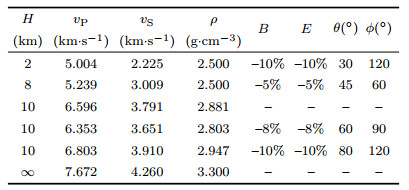
Table 4 provides the crustal model for the synthetic data test. The horizontal slowness is 0.0618 s·km-1. The crustal model includes low-velocity layer, high-velocity layer and sedimentary thin layer. Note that: (1) in this test, we assume the isotropic structure as known quantity. The stratification of anisotropy is the same as that of velocity. We only invert for the anisotropic parameters, including those in the isotropic layer. (2) All initial anisotropic parameters are set to zero. (3) The magnitude of P and S anisotropy remain equal, and the value ranges from-20% to 0%. The trend of symmetry axis ranges from 0° to 90°, while the plunge ranges from 0° to 360°. (4) The swarm size is 50 and the maximum number of iterations is 100.
|
|
Table 4 Anisotropic model parameters used for synthetic data test |
The results are showed in Fig. 8. The correlation coefficient between the RF data in Fig. 8a and the predicted RF in Fig. 8b is close to 1.0. The red dots in Fig. 8f denote the curve of convergence. In fact, the misfit is acceptable after about 50 iterations. The inverted parameters in Fig. 8(c-e) are basicly the same as the testing model in Table 4. The test results show that our method can correctly recover the depth-dependent anisotropic parameters from the RF data without noise, when the isotropic model is known or predetermined. The observed RF data contain the lateral scattering and other noise, which increases the difficulties for seismic anisotropy study (Savage, 1998). The spatial orientation of the lateral scattering and other noise may manifest a certain degree of randomness, while the wavefield pattern of seismic anisotropy shows strong traceability along the backazimuth. The results from Qi et al. (2016) demonstrate that curvelet denoising can significantly improve the traceability of the two-dimensional RF wavefield, and wavefield reconstruction using compressive sensing can recover a certain amount of missing data. There is no doubt that such technique is useful for seismic anisotropic study.

|
Fig. 8 Numerical test of the inversion of RF for seismic anisotropy (a) 'True' RF; (b) Predicted RF; (c) Trend of anisotropy; (d) Plunge of anisotropy; (e) Isotropic velocity model and magnitude of anisotropy; (f) Misfit between 'true' and predicted RF. 'sum' denotes the summation over all backazimuths; 'Ani' denotes magnitude of anisotropy; colored dots denote the misfit for each model; red dots denote the global misfit; shaded area represents isotropic layer. |
Qi et al. (2016) has already applied this method to the RF data recorded by permanent Station CTAO (Lat:-20.0882°N, Lon: 146.2545°E, Code: IU), which is located in the northeast of Australia and belongs to IRIS global seismographic network. The geographic location of Station CTAO and its tectonic background is showed in Fig. 9. We take the denoised data from this station for the real data test using our inversion method.

|
Fig. 9 Geographic location of Station CTAO and its tectonic background (modified from Ford et al., 2010) Black solid lines outline the major tectonic provinces in Australia; western regions with inclined lines indicate Archean cratons; northern and southern regions with horizontal lines indicate Proterozoic cratons; eastern regions with dots indicate Phanerozoic basements; black triangles denote IRIS stations, while red triangle represents station CTAO in this study. |
The time-domain iterative deconvolution method (Ligorr' la and Ammon, 1999) is used to estimate the RF data. The RF data without denoising is showed in Qi et al. (2016). The parameters of data processing are as follows: (1) the Gaussian coefficient of 2.5 is used. (2) The backazimuthal interval of wavefield reconstruction is 1°. The processed data is showed in Fig. 10a. Note that, the data has been averaged by the backazimuthal interval of 10°.

|
Fig. 10 Inversion of anisotropy from RF at Station CTAO (a) Observed RF; (b) Predicted RF; (c) Trend of anisotropy; (d) Plunge of anisotropy; (e) Isotropic velocity model and magnitude of anisotropy; (f) Misfit between observed and predicted RF. |
The inversion takes two steps: (1) the isotropic structure is first determined from the average waveform of all backazimuths. (2) We simplify the model to five layers for the crust. Note that, the isotropic structure is fixed during the inversion of anisotropy, and the inversion does not involve the structure below the Moho.
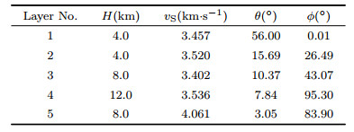
The predicted RF wavefield is showed in Fig. 10b, and the inverted anisotropic parameters are given in Fig. 10(c-e) and Table 5. The crustal thickness beneath Station CTAO is 36 km in our study, which is generally consistent with the result of 34 km from Chevrot and van der Hilst (2000) by using the H-κ stacking method.
|
|
Table 5 The plunge and trend of the slow-axis crustal anisotropy beneath Station CTAO |
From Fig. 10(a, b), we find that the major backazimuthal pattern is well recovered. Note that, the misfit function is based on waveform cross-correlation, the inversion is therefore more sensitive to the phase than amplitude of the data. The differences between the data and prediction are reasonable. On one hand, the lateral stratified crustal model is insufficient to fully interpret the data from the three-dimensional wavefield. On the other hand, we did not include seismic anisotropy of the upper mantle. The magnitude of anisotropy beneath Station CTAO is showed in Fig. 10e. The anisotropy is relatively weak in the shallow crust and strong in the deeper crust. The maximal value of the magnitude is comparable to the previous results (~20%) in other regions. (Sherrington et al., 2004; Tian et al., 2008).
The plunge and trend of anisotropic symmetry axis is showed in Fig. 10(c, d) and Table 5. Since there is no previous report regarding the stratified crustal anisotropy, we cannot provide comparable evidence from other RF studies. However, our result shows agreement with seismic anisotropy from surface wave studies, which is summarized as follows:
(1) The plunge of slow axis tends to lie vertically as the depth increases. It implies that the anisotropic fabric is horizontally oriented in the middle and lower crust, and the wave velocity is faster in the horizontal than in the vertical direction, which agrees with the radial anisotropy that the SH velocity is faster than SV above 200 km in the lithosphere (Debayle and Kennett, 2000).
(2) The trend of slow axis approximately lies to the EW direction in the lower crust (layer No.4 and 5). The fast direction is approximately in the NS direction, which agrees with the results of the azimuthal anisotropy from Rayleigh wave studies (Debayle and Kennett, 2000; Simons and van der Hilst, 2003).
4 CONCLUSION AND DISCUSSIONIn this paper, we investigate the RF wavefield from stratified crustal anisotropic models and evaluate the impact of anisotropic parameters at different depths on the backazimuthal pattern of RF wavefield, which provides a new theoretical basis for seismic anisotropy study. We develop a global inversion method for extracting stratified anisotropic models based on the particle swarm algorithm. Numerical and real data test show that, our method is capable of recovering the depth-dependent anisotropic parameters from the RF data. Our conclusions are as follows:
(1) The RF wavefield patterns between the fast-axis and slow-axis anisotropy are different. The anisotropic pattern is more sensitive to the trend of symmetry axis. The influence of seismic anisotropy on the transverse component is stronger than that on the radial component. The backazimuthal pattern of Ps conversion from the interface between two consecutive anisotropic layers is the combination of effects from both layers, and the intensity of the pattern depends on the contrast of anisotropic parameters in the two layers. The reverberations from the sedimentary layer will make interference to the RF wavefield. The anisotropic thin layer can lead to the separation of converted phases, but the anisotropic effect of the corresponding multiples is reduced. The theoretical research shows that the polarization analysis based on single phase has limitations in the study of the stratified anisotropy.
(2) The results from the numerical test show that our method can correctly recover the depth-dependent anisotropic parameters from the RF data, as long as the isotropic velocity model is well predetermined. Since RF is not sensitive to the absolute velocity, the estimation of isotropic structure may consider the joint inversion of RF and data from other observations. In addition, it may be helpful to include the multiples into the inversion.
(3) The tests of the observed data show that the curvelet denoising can reduce the lateral scattering and other noise in the data, and the wavefield reconstruction can provide data with complete backazimuthal coverage. These techniques are important for the extracting of depth-dependent anisotropic parameters and minimizing the nonuniqueness of the inversion.
(4) Note that, the curvelet denoising does not remove the three-dimensional effect of the data. Theoretically speaking, including the multiples into the inversion may be helpful. Due to the low SNR and the amplification effect along their paths, the identification of the anisotropic pattern for the multiples remains difficult.
| [] | Audet P. 2015. Layered crustal anisotropy around the San Andreas Fault near Parkfield, California. J. Geophys. Res. , 120 (5) : 3527-3543. DOI:10.1002/2014JB011821 |
| [] | Babuska V, Cara M. 1991. Seismic Anisotropy in the Earth[M]. Netherlands: Kluwer Academic Publishers . |
| [] | Backus G E. 1965. Possible forms of seismic anisotropy of the uppermost mantle under oceans. J. Geophys. Res. , 70 (14) : 3429-3439. DOI:10.1029/JZ070i014p03429 |
| [] | Beaumont C, Jamieson R A, Nguyen M H, et al. 2001. Himalaya tectonics explained by extrusion of a low-viscosity crustal channel coupled to focused surface denudation. Nature , 414 (6865) : 738-742. DOI:10.1038/414738a |
| [] | Chen X F. 1993. A systematic and efficient method of computing normal modes for multilayered half-space. Geophys. J. Int. , 115 (2) : 391-409. DOI:10.1111/gji.1993.115.issue-2 |
| [] | Chevrot S, van der Hilst R D. 2000. The Poisson ratio of the Australian crust:geological and geophysical implications. Earth Planet. Sci. Lett. , 183 (1-2) : 121-132. DOI:10.1016/S0012-821X(00)00264-8 |
| [] | Clerc M, Kennedy J. 2002. The particle swarm-explosion, stability, and convergence in a multidimensional complex space. IEEE Transactions on Evolutionary Computation , 6 (1) : 58-73. DOI:10.1109/4235.985692 |
| [] | Crampin S. 1987. Geological and industrial implications of extensive-dilatancy anisotropy. Nature , 328 (6130) : 491-496. DOI:10.1038/328491a0 |
| [] | Debayle E, Kennett B L N. 2000. Anisotropy in the Australasian upper mantle from Love and Rayleigh waveform inversion. Earth Planet. Sci. Lett. , 184 (1) : 339-351. DOI:10.1016/S0012-821X(00)00314-9 |
| [] | Eberhart R C, Kennedy J. 1995. A new optimizer using particle swarm theory. //Proceedings of the Sixth International Symposium on Micro Machine and Human Science. Nagoya: IEEE, 39-43. |
| [] | Eberhart R C, Shi Y H. 1998. Comparison between genetic algorithms and particle swarm optimization. //Proceedings of the 7th International Conference on Evolutionary Programming. San Diego, California, USA: Springer, 611-616. |
| [] | Erickson J. 2002. Anisotropic crustal structure inversion using a niching genetic algorithm: A feasibility study[Master thesis]. Tucson: Universityof Arizona. |
| [] | Fang L H, Wu J P. 2009. Effects of dipping boundaries and anisotropic media on receiver functions. Progress in Geophys. , 24 (1) : 42-50. |
| [] | Ford H A, Fischer K M, Abt D L, et al. 2010. The lithosphere-asthenosphere boundary and cratonic lithospheric layering beneath Australia from Sp wave imaging. Earth Planet. Sci. Lett. , 300 (3-4) : 299-310. DOI:10.1016/j.epsl.2010.10.007 |
| [] | Frederiksen A W, Bostock M G. 2000. Modelling teleseismic waves in dipping anisotropic structures. Geophys. J. Int. , 141 (2) : 401-412. DOI:10.1046/j.1365-246x.2000.00090.x |
| [] | Frederiksen A W, Folsom H, Zandt G. 2003. Neighbourhood inversion of teleseismic Ps conversions for anisotropy and layer dip. Geophys. J. Int. , 155 (1) : 200-212. DOI:10.1046/j.1365-246X.2003.02043.x |
| [] | Girardin N, Farra V. 1998. Azimuthal anisotropy in the upper mantle from observations of P-to-S converted phases:application to southeast Australia. Geophys. J. Int. , 133 (3) : 615-629. DOI:10.1046/j.1365-246X.1998.00525.x |
| [] | Hassan R, Cohanim B, De Weck O, et al. 2005. A comparison of particle swarm optimization and the genetic algorithm. //Proceedings of the 46thAIAA/ASME/ASCE/AHS/ASC Structures, Structural Dynamics and Materials Conference. Austin, Texas: AIAA. |
| [] | Leidig M, Zandt G. 2003. Modeling of highly anisotropic crust and application to the Altiplano-Puna volcanic complex of the central Andes. J. Geophys. Res. , 108 (B1) : ESE 5-1-ESE 5-15. DOI:10.1029/2001JB000649 |
| [] | Levin V, Park J. 1997. P-SH conversions in a flat-layered medium with anisotropy of arbitrary orientation. Geophys. J. Int. , 131 (2) : 253-266. DOI:10.1111/gji.1997.131.issue-2 |
| [] | Ligorr′ la J P, Ammon C J. 1999. Iterative deconvolution and receiver-function estimation. Bull. Seism. Soc. Am. , 89 (5) : 1395-1400. |
| [] | Liu H F, Niu F L. 2012. Estimating crustal seismic anisotropy with a joint analysis of radial and transverse receiver function data. Geophys. J. Int. , 188 (1) : 144-164. DOI:10.1111/gji.2012.188.issue-1 |
| [] | Liu Q Y, Shao X Z. 1985. Study on the dynamic characteristics of PS converted waves. Acta Geophysica Sinica , 28 (3) : 291-302. |
| [] | Liu Q Y, Wang J, Chen J H, et al. 2007. Seismogenic tectonic environment of 1976 great Tangshan earthquake:results given by dense seismic array observations. Earth Science Frontiers , 14 (6) : 205-213. DOI:10.1016/S1872-5791(08)60012-3 |
| [] | Liu Q Y, van der Hilst R D, Li Y, et al. 2014. Eastward expansion of the Tibetan Plateau by crustal flow and strain partitioning across faults. Nature Geoscience , 7 (5) : 361-365. DOI:10.1038/ngeo2130 |
| [] | Lloyd G E, Butler R W H, Casey M, et al. 2009. Mica, deformation fabrics and the seismic properties of the continental crust. Earth Planet. Sci. Lett. , 288 (1-2) : 320-328. DOI:10.1016/j.epsl.2009.09.035 |
| [] | Mart′ llnez J L F, Gonzalo E G, álvarez J P F, et al. 2010. PSO:a powerful algorithm to solve geophysical inverse problems:application to a 1D-DC resistivity case. Journal of Applied Geophysics , 71 (1) : 13-25. DOI:10.1016/j.jappgeo.2010.02.001 |
| [] | McNamara D E, Owens T J. 1993. Azimuthal shear wave velocity anisotropy in the Basin and Range province using Moho Ps converted phases. J. Geophys. Res. , 98 (B7) : 12003-12017. DOI:10.1029/93JB00711 |
| [] | Nagaya M, Oda H, Akazawa H, et al. 2008. Receiver functions of seismic waves in layered anisotropic media:Application to the estimate of seismic anisotropy. Bull. Seism. Soc. Am. , 98 (6) : 2990-3006. DOI:10.1785/0120080130 |
| [] | Nicolas A, Christensen N I. 1987. Formation of anisotropy in upper mantle peridotites-A review. //Froidevaux C, Fuchs K, eds. Composition, Structure and Dynamics of the Lithosphere-Asthenosphere System. Washington DC: AGU, 111-123. |
| [] | Okaya D A, McEvilly T V. 2003. Elastic wave propagation in anisotropic crustal material possessing arbitrary internal tilt. Geophy. J. Int. , 153 (2) : 344-358. DOI:10.1046/j.1365-246X.2003.01896.x |
| [] | Ozacar A A, Zandt G. 2004. Crustal seismic anisotropy in central Tibet:Implications for deformational style and flow in the crust. Geophys. Res. Lett. , 31 (23) : L23601. |
| [] | Park J, Yu Y. 1992. Anisotropy and coupled free oscillations:simplified models and surface wave observations. Geophys. J. Int. , 110 (3) : 401-420. DOI:10.1111/gji.1992.110.issue-3 |
| [] | Porter R, Zandt G, McQuarrie N. 2011. Pervasive lower-crustal seismic anisotropy in Southern California:Evidence for under platedschists and active tectonics. Lithosphere , 3 (3) : 201-220. DOI:10.1130/L126.1 |
| [] | Qi S H, Liu Q Y, Chen J H, et al. 2009. Wenchuan earthquake Ms8. 0:Preliminary study of crustal anisotropy on both sides of the Longmenshan faults. Seismology and Geology , 31 (3) : 377-388. |
| [] | Qi S H, Liu Q Y, Chen J H, et al. 2016. Attenuation of noise in receiver functions using curvelet transform. Chinese J. Geophys. , 59 (3) : 884-896. DOI:10.6038/cjg20160311 |
| [] | Rabbel W, MooneyW D. 1996. Seismic anisotropy of the crystalline crust:What does it tell us?. Terra Nova , 8 (1) : 16-21. DOI:10.1111/ter.1996.8.issue-1 |
| [] | Rümpker G, Kaviani A, Latifi K. 2014. Ps-splitting analysis for multilayered anisotropic media by azimuthal stacking and layer stripping. Geophys. J. Int. , 199 (1) : 146-163. DOI:10.1093/gji/ggu154 |
| [] | Savage M K. 1998. Lower crustal anisotropy or dipping boundaries? Effects on receiver functions and a case study in New Zealand. J. Geophys. Res. , 103 (B7) : 15069-15087. DOI:10.1029/98JB00795 |
| [] | Savage M K. 1999. Seismic anisotropy and mantle deformation:what have we learned from shear wave splitting. Rev. Geophys. , 37 (1) : 65-106. DOI:10.1029/98RG02075 |
| [] | Schulte-Pelkum V, Mahan K H. 2014. A method for mapping crustal deformation and anisotropy with receiver functions and first results from USArray. Earth Planet. Sci. Lett. , 402 : 221-233. DOI:10.1016/j.epsl.2014.01.050 |
| [] | Shaw R, Srivastava S. 2007. Particle swarm optimization:A new tool to invert geophysical data. Geophysics , 72 (2) : F75-F83. DOI:10.1190/1.2432481 |
| [] | Sherrington H F, Zandt G, Frederiksen A. 2004. Crustal fabric in the Tibetan Plateau based on waveform inversions for seismic anisotropy parameters. J. Geophys. Res. , 109 : B02312. |
| [] | Shi X M, Xiao M, Fan J K, et al. 2009. The damped PSO algorithm and its application for magnetotelluric sounding data inversion. Chinese J. Geophys. , 52 (4) : 1114-1120. DOI:10.3969/j.issn.0001-5733.2009.04.029 |
| [] | Shi Y, Eberhart R. 1998. A modified particle swarm optimizer. //Proceedings of the 1998 IEEE International Conference on Evolutionary Computation Proceedings, 1998. IEEE World Congress on Computational Intelligence. Anchorage, AK: IEEE, 69-73. |
| [] | Silver P G, Chan W W. 1991. Shear wave splitting and subcontinental mantle deformation. J. Geophys. Res. , 96 (B10) : 16429-16454. DOI:10.1029/91JB00899 |
| [] | Simons F J, van der Hilst R D. 2003. Seismic and mechanical anisotropy and the past and present deformation of the Australian lithosphere. Earth Planet. Sci. Lett. , 211 (3-4) : 271-286. DOI:10.1016/S0012-821X(03)00198-5 |
| [] | Tian B F, Li J, Wang W M, et al. 2008. Crust anisotropy of Taihangshan mountain range in north China inferred from receiver functions. Chinese J. Geophys. , 51 (5) : 1459-1467. |
| [] | Vinnik L P, Farra V, Romanowicz B. 1989. Azimuthal anisotropy in the earth from observations of SKS at GEOSCOPE and NARS broadband stations. Bull. Seism. Soc. Am. , 79 (5) : 1542-1558. |
| [] | Ward D, Mahan K, Schulte-Pelkum V. 2012. Roles of quartz and mica in seismic anisotropy of mylonites. Geophys. J. Int. , 190 (2) : 1123-1134. DOI:10.1111/gji.2012.190.issue-2 |
| [] | Weiss T, Siegesmund S, Rabbel W, et al. 1999. Seismic velocities and anisotropy ofthe lower continental crust: A review. //Seismic Exploration of the Deep Continental Crust. Basel: Birkh-user, 97-122. |
| [] | Xu Z, Xu M J, Wang L S, et al. 2006. A study on crustal anisotropy using P to S converted phase of the receiver function:Application to Ailaoshan-Red River fault zone. Chinese J. Geophys. , 49 (2) : 438-448. |
| [] | Yao C. 1989. The splitting of the teleseismic PS waves propagating through cracked solids. Earthquake Research in China , 5 (1) : 38-47. |
| [] | Yao C, Cai M G. 2009. Analytical expression of TI elastic tensor with arbitrary orientation. Chinese J. Geophys. , 52 (9) : 2345-2348. DOI:10.3969/j.issn.0001-5733.2009.09.019 |
| [] | Yao C, Hao C T, Zhang G L. 2016. A study of synthetic seismograms for SKS-wave response to crustal fractured-induce anisotropy. Chinese J. Geophys. , 59 (7) : 2498-2509. DOI:10.6038/cjg20160715 |
| [] | Yue B B, Peng Z M, Hong Y G, et al. 2009. Wavelet inversion of pre-stack seismic angle-gather based on particle swarm optimization algorithm. Chinese J. Geophys. , 52 (12) : 3116-3123. DOI:10.3969/j.issn.0001-5733.2009.12.021 |
| [] | Zandt G, Gilbert H, Owens T J, et al. 2004. Active foundering of a continental arc root beneath the southern Sierra Nevada in California. Nature , 431 (7004) : 41-46. DOI:10.1038/nature02847 |
| [] | Zhu T, Li X F, Li Y Q, et al. 2011. Seismic scalar wave equation inversion based on an improved particle swarm optimization algorithm. Chinese J. Geophys. , 54 (11) : 2951-2959. DOI:10.3969/j.issn.0001-5733.2011.11.025 |