 2017, Vol. 60


With the increasingly wide use of airborne electromagnetic (AEM) in the mineral, oil and gas, ground water, environmental and engineering exploration (Lei et al., 2006; Yin et al., 2015), AEM data interpretation and imaging become more and more important. However, in the imaging techniques of AEM some parameters like imaging depth can only be determined empirically (Huang and Rudd, 2008) but cannot be solved clearly. In this paper, we discuss a fundamental airborne phenomenon of the electromagnetic (EM) diffusion by showing how the EM fields propagate and diffuse in the earth; and based on this concept, we try to determine parameters like the imaging depth for time-domain AEM data imaging.
Based on the Ampere's law, the electric current flowing in the transmitting loop of a time-domain AEM system generates a primary magnetic field. When the transmitting current is switched off, the primary field vanishes. This change induces the eddy current inside the earth according to Faraday's law. The eddy current propagates through the earth in a diffusive way, with its distribution becoming wider and its strength decaying with time, which is called "electromagnetic diffusion".
Visualization of EM diffusion for a time-domain AEM system is important for understanding the transient process of an AEM system. The current distribution and diffusion features can provide effective means to evaluate depth of exploration (Chen et al., 2014), EM footprint (Beamish, 2003; Yin et al., 2014) and diffusion depth (Beamish, 2004) etc., which can further help in AEM system design and data processing.
In the past, many geophysicists have worked on EM diffusion for ground transient EM systems. Lewis and Lee (1978) studied the transient electric fields in the underground for a loop laid on a homogeneous halfspace. Nabighian (1979) proposed that the transient EM field induced by a step function observed over a conductive half-space or a layered earth can be represented by a simple current filament of the same shape as the transmitter loop, moving downward and outward with a decreasing velocity and diminishing amplitude, resembling a system of "smoke rings". Hoversten and Morrison (1982) showed that the induced electric field within a four-layer model by a repetitive current waveform in a circular loop transmitter forms a single smoke ring. More recently, Wang (2002) examined the EM smoke ring in a transversely isotropic medium. Other 2D forward modeling (Yan et al., 2002) has also presented the EM current system in a static format of 2D contours or vectors. Researches have also been worked on airborne EM diffusion. Yin and Hodges (2005) investigated the EM diffusion in the half-space earth for a frequency-domain AEM system. Then Yin and Hodges (2007) further extended the half-space model to more complicated structures of an anisotropic earth and 2D and 3D structures. However, most previous studies on time-domain EM diffusion or smoke ring are based on the static presentation for ground EM systems, where the dynamic features of EM diffusion were not visible. Yin and Hodges (2007) incorporated a time factor eiωt into frequency-domain EM field and displayed EM diffusion in a 3D animated flux of vectors or contours, but their presentation does not reveal the true EM smoke ring because instead of the time they assume the EM phase changes, so that the EM field varies periodically.
AEM imaging has become the most routine and popular procedure in AEM data processing due to its simplicity and efficiency. However, the determination of imaging depth for time-domain AEM data has confused geophysical community for many years. For the imaging algorithms like CDI/CDT (Huang and Rudd, 2008; Li et al., 2010; Zhu et al., 2010; Chen and Duan, 2012; Mao, 2013), the apparent resistivity obtained from a look-up table is empirically plotted against an imaging depth close to half of the diffusion depth, but nobody can explain how the imaging depth is obtained.
In this paper, we study the true EM diffusion and smoke ring for an AEM system by investigating the propagation of EM field inside the earth with time. We first calculate the frequency-domain EM field inside the earth by the continuation algorithm developed by Yin and Maurer (2001). Then, we transform the EM field into time-domain via a Fourier transform and display the time-varying induced current in an animated dynamic format from which the EM smoke ring is clearly distinguished. Finally, we try to apply the EM smoke ring concept to establish a relationship between the diffusion depth and the imaging depth for AEM imaging. We take a homogeneous half-space model and a two-layer earth model as examples to investigate the diffusion for an AEM system and consider both vertical and horizontal magnetic transmitting dipoles.
2 MODELING METHODOLOGYFigure 1 shows an AEM transmitter over a layered isotropic earth. A coordinate system is established with x-and y-axis located at the earth's surface and z-axis positive downwards. For simplicity, only a vertical magnetic dipole is presented in Fig. 1. The dipole is located at (0, 0, -h0), where h0 denotes the altitude of the dipole.

|
Fig. 1 A vertical magnetic dipole over a layered earth |
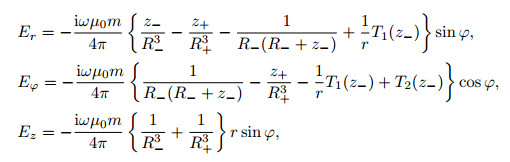
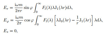
After Weidelt (1991), the radial, tangential and vertical electric field in the air (r, φ, z) for a horizontal magnetic dipole are
|
(1) |
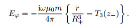
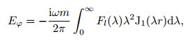
while for a vertical magnetic dipole, the tangential electric field is
|
(2) |
In the above equations, i is the imaginary unit, ω is the angular frequency, μ0 is the permeability, m is the dipole moment, 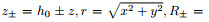

|
(3) |
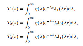
where J0(λr) and J1(λr) are Bessel functions of order 0 and 1; η(λ) is the kernel function related to the spatial wavenumber λ and the earth parameters (Weidelt, 1991). Following the procedure developed by Yin and Hodges (2005), we can obtain the electric field for a horizontal magnetic dipole at location (r, φ, z) in layer l of the earth with
|
(4) |
while for a vertical magnetic dipole, we have
|
(5) |
where Fl(λ) is the kernel function based on the continuation boundary condition. A recursive calculation of this function and the numerical algorithm for the above integrals can be found from Weidelt (1991).
After obtaining the EM field in polar coordinate system, we project them onto the x-and y-axis to obtain the EM field in the Cartesian coordinate system. The current density inside the earth is obtained by Ohm's law: J = σE, where σ denotes the earth's conductivity.
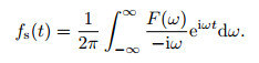
After obtaining the frequency-domain EM field, we use the Fourier transform to calculate the time-domain EM field (Yin et al., 2013):
|
(6) |
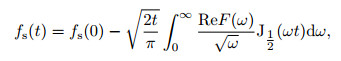
Reformulating Eq.(6), we obtain
|
(7) |
where 
To visualize EM diffusion for a time-domain AEM system, we calculate the current density inside the earth induced by a step pulse for 900 channels from 0.002 ms to 5.0 ms. Then, we display the current distribution as 3D time-varying contours to visualize EM diffusion. We first choose a homogeneous half-space model with a resistivity of 100 Ωm from Yin and Hodges (2007) to investigate the differences between time-and frequencydomain EM diffusions. Fig. 2 shows 3D view of the electric field and current density for horizontal and vertical magnetic dipoles. The decay time is 0.5 ms. The current density is displayed as contours, while the electric field is displayed as arrows, with the length of the arrows denoting the field strength, while the middle point of each arrow denoting the location where the electric field is calculated. We have blanked out the quarter corner at lower right to view the internal structures of the induced current.

|
Fig. 2 Distribution of current density inside the earth for a vertical and a horizontal magnetic dipole over a homogeneous half-space at the decay time of 0.5 ms Current density at the earth surface for (a) vertical magnetic dipole and (b) horizontal magnetic dipole; Current density inside the earth for (c) vertical magnetic dipole and (d) horizontal magnetic dipole. |
From Fig. 2, we can see that 1) for a vertical magnetic dipole, the underground current forms only one circle, corresponding to the polarity of the magnetic flux for a vertical magnetic dipole, injecting into the earth; 2) for a horizontal magnetic dipole, however, the underground current forms two circles stacked in the middle, corresponding to the two polarities of the magnetic flux for a horizontal magnetic dipole, injecting into or ejected from the earth; 3) there exists no vertical current in a layered isotropic earth. The currents for both horizontal and vertical magnetic dipoles flow horizontally.
To differentiate the time-domain smoke rings from the frequency-domain ones, we display in Fig. 3 the horizontal current density in the same homogeneous half-space of 100 Ωm. Comparison of Fig. 3 with Fig. 8 of Yin and Hodges (2007) shows that whereas the time-domain EM smoke ring diffuses with time outward and downward, its strength decays; the frequency-domain smoke ring diffuses, but its strength and polarities change periodically. Thus, we draw the conclusion that the time-domain EM smoke ring presented in this paper demonstrates the true EM diffusion, because the EM field propagates outward and downward, decays with time, and becomes more diffuse; while the frequency-domain smoke ring presented by Yin and Hodges (2007) shows only the periodical polarity and amplitude change of EM fields. The variation in frequency-domain resulted from the introduction of the phase term eiωt that is multiplied with the complex EM field.

|
Fig. 3 Current density in contours for a vertical magnetic dipole over a homogeneous half-space of 100 Ωm (a) 900 Hz for frequency-domain; (b) Time-domain at the decay time of 0.5 ms. |

|
Fig. 8 Relationship between imaging depth and diffusion depth for different homogeneous half-space models (a) Vertical magnetic dipole; (b) Horizontal magnetic dipole. |
Further, we study the EM diffusion for a layered earth model. We assume a two-layer earth with a top layer of 50 Ωm over an underlying half-space of 100 Ωm. The overburden has a thickness of 200 m. The altitude of the magnetic dipole is 30 m. Fig. 4 shows the 3D animated current distribution for a vertical magnetic dipole above the two-layer earth. From the figure, one sees that 1) the current distribution is closely correlated with the resistivity interfaces. There exists a sharp change of current at the boundary between the first and second layer, so that the resistivity interface is clearly distinguished from the current distribution. This is because at the layer interface, though the vertical current is continuous (both zero), but the horizontal current is discontinuous, Fig. 3 Current density in contours for a vertical magnetic dipole over a homogeneous half-space of 100 Ωm (a) 900 Hz for frequency-domain; (b) Time-domain at the decay time of 0.5 ms. resulting in the discontinuity of total current; 2) the EM field in the conductive top layer propagates more slowly but decays faster than in the resistive underlying halfspace. This implies that in the practical AEM survey, to detect the targets under a conductive overburden, the later time channel signal is needed. To conduct the research more directly, only half-space and layered earth models are discussed in this section. But it needs to be pointed out that, the EM diffusion law still remains in complicated electrical media.

|
Fig. 4 Current density in contours for a vertical magnetic dipole over a two-layer earth model at the decay time of 0.5 ms |
In this section, we further investigate the EM diffusion by extracting the current filament from the underground induced current system—the EM smoke ring. The EM diffusion depth for time t equals 

|
Fig. 5 Center current and edge current for current rings of a horizontal magnetic dipole |
|
(8) |
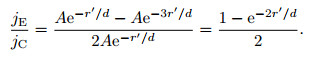
Assuming that the radius of a smoke ring r' is 0.55 times the diffusion depth d, we have
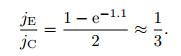
|
(9) |
Thus, we take a third of the maximum current density as the threshold for extracting the smoke ring for the vertical magnetic dipole.
Figure 6 shows smoke rings for vertical and horizontal transmitting dipoles induced in the homogeneous half-space earth of 100 Ωm at the decay time of 0.5 ms. From Fig. 6, we can see that 1) the induced current for a vertical magnetic dipole forms a circular smoke ring; 2) for a horizontal magnetic dipole, the current forms two stacked rings with the maximum current located under the transmitting dipole; 3) the induced current for both vertical and horizontal magnetic dipoles propagates downward and outward with time, becoming wider and more diffuse, the amplitude of the current attenuates with decaying time.

|
Fig. 6 Current rings for (a) a vertical magnetic dipole and (b) a horizontal magnetic dipole over a homogeneous half-space of 100 Ωm at the decay time of 0.5 ms |
Figure 7 shows the smoke ring for the vertical magnetic dipole over the two-layer earth model given in Fig. 4, and the decay time is 1.0 ms. From the figure, we can see that 1) there exists only a single smoke ring even for a layered earth. This is in opposite to the frequency-domain smoke ring shown by Yin and Hodges(2005, 2007); 2) the smoke ring first exists only in the top layer, with the increase of decay time, it Fig. 7 Current ring for a vertical magnetic dipole over a two-layer earth model at the decay time of 1.0 ms diffuses outward and propagates downward into the second layer; 3) in the conductive top layer the smoke ring propagates slowly but decays fast, but in the resistive underlying half-space it propagates fast but decays slowly. Due to big difference of traveling time, the partial smoke ring in the underlying half-space looks smaller than in the top layer.

|
Fig. 7 Current ring for a vertical magnetic dipole over a two-layer earth model at the decay time of 1.0 ms |
In airborne electromagnetic, imaging is a very effective and efficient way to interpret AEM data. The most frequently used techniques include conductivity-depth-imaging (CDI) and conductivity-depth-transform (CDT). To image underground structures from the AEM data, we generally take the resistivity of a homogeneous half-space that produces the same EM signal as apparent resistivity and plot it against the imaging depth that is until now empirically determined and very close to half of the diffusion depth. However, nobody knows how this imaging depth is obtained. In this section, starting from the EM smoking ring, we establish a relationship between the depth of maximum current and the diffusion depth. From this relationship, we can obtain the imaging depth for time-domain AEM data.
Figure 8 shows the relationship between the depth of maximum current density and the diffusion depth for different homogeneous half-space models. The resistivity of these four models is respectively 25, 50, 75, and 100 Ωm. It is seen that the depth for the maximum current density maintains a linear relationship with the diffusion depth for both vertical and horizontal magnetic dipoles with a slope of about 0.55, meaning that the depth of the maximum current density is roughly at 0.55 times the diffusion depth 
By showing the underground current and electric field as 3D animated contours and time-varying vectors, the EM diffusion and smoke ring are clearly observed. In a homogeneous half-space, the induced current for a vertical magnetic dipole forms a single ring, propagating with time downward and outward, becoming wider and more diffuse; while for a horizontal magnetic dipole, the underground current forms two stacked rings. Even in the layered earth, the EM field forms only a single smoke ring, propagating in the top layer first and then into the underlying layers. This is in opposite to the case in frequency-domain (Yin and Hodges, 2007). In a conductive layer, the EM field propagates slowly but decays fast, while in a resistive layer it propagates fast but decays slowly. By analyzing the relationship between the depth of maximum current and the diffusion depth, we have confirmed the imaging depth commonly used in AEM imaging to be 0.55 times the diffusion depth. An animated EM smoke ring offers more information than a static contour. More work can be done on extending EM diffusion features to study the footprint, resolution, and exploration depth of an AEM system. This will be our future research focus.
ACKNOWLEDGMENTSThe research of this paper is financially supported by the Key Program of the National Natural Science Foundation of China (41530320), Natural Science Foundation (41274121), China Natural Science Foundation for Young Scientists (41404093) and Projects on the Development of the Key Equipment of Chinese Academy of Sciences (ZDYZ2012-1-03, 20130523MTEM05).
| [] | Beamish D. 2003. Airborne EM footprints. Geophysical Prospecting , 51 (1) : 49-60. DOI:10.1046/j.1365-2478.2003.00353.x |
| [] | Beamish D. 2004. Airborne EM skin depths. Geophysical Prospecting , 52 (5) : 439-449. DOI:10.1111/gpr.2004.52.issue-5 |
| [] | Chen B, Mao L F, Liu G D. 2014. The estimated prospecting depth of CHTEM-I system by the method of diffusion electric field. Chinese J. Geophys. , 57 (1) : 303-309. DOI:10.6038/cjg20140126 |
| [] | Chen X H, Duan N J. 2012. Study on fast imaging of airborne time-domain electromagnetic data. Progress in Geophys. , 27 (5) : 2123-2127. DOI:10.6038/j.issn.1004-2903.2012.05.037 |
| [] | Hoversten G M, Morrison H F. 1982. Transient fields of a current loop source above a layered earth. Geophysics , 47 (7) : 1068-1077. DOI:10.1190/1.1441370 |
| [] | Huang H P, Rudd J. 2008. Conductivity-depth imaging of helicopter-borne TEM data based on a pseudolayer half-space model. Geophysics , 73 (3) : F115-F120. DOI:10.1190/1.2904984 |
| [] | Lei D, Hu X Y, Zhang S F. 2006. Development status of airborne electromagnetic. Contributions to Geology and Mineral Resources Research , 21 (1) : 40-44. |
| [] | Lewis R, Lee T. 1978. The transient electric fields about a loop on a halfspace. Exploration Geophysics , 9 (4) : 173-177. DOI:10.1071/EG978173 |
| [] | Li Y X, Qiang J K, Tang J T. 2010. A research on 1-D forward and inverse airborne transient electromagnetic method. Chinese J. Geophys. , 53 (3) : 751-759. DOI:10.3969/j.issn.0001-5733.2010.03.031 |
| [] | Mao L F. 2013. Conductivity-depth imaging algorithm for central-loop helicopter TEM. CT Theory and Applications , 22 (3) : 429-437. |
| [] | Nabighian M N. 1979. Quasi-static transient response of a conducting half-space-An approximate representation. Geophysics , 44 (10) : 1700-1705. DOI:10.1190/1.1440931 |
| [] | Wang T. 2002. The electromagnetic smoke ring in a transversely isotropic medium. Geophysicss , 67 (6) : 1779-1789. DOI:10.1190/1.1527078 |
| [] | Weidelt P. 1991. Introduction into electromagnetic sounding. Lecture manuscript, Technical University of Braunschweig. |
| [] | Yan S, Chen M S, Fu J M. 2002. Direct time-domain numerical analysis of transient electromagnetic fields. Chinese J. Geophys. , 45 (2) : 275-284. |
| [] | Yin C, Maurer H M. 2001. Electromagnetic induction in a layered earth with arbitrary anisotropy. Geophysics , 66 (5) : 1405-1416. DOI:10.1190/1.1487086 |
| [] | Yin C C, Hodges G. 2005. Four dimensional visualization of EM fields for a helicopter EM system. //75th Annual International Meeting, SEG, Expanded Abstracts, 595-598. |
| [] | Yin C C, Hodges G. 2007. 3D animated visualization of EM diffusion for a frequency-domain helicopter EM system. Geophysics , 72 (1) : F1-F7. DOI:10.1190/1.2374706 |
| [] | Yin C C, Huang W, Ben F. 2013. The full-time electromagnetic modeling for time-domain airborne electromagnetic systems. Chinese J. Geophys. , 56 (9) : 3153-3162. DOI:10.6038/cjg20130928 |
| [] | Yin C C, Huang X, Liu Y H, et al. 2014. Footprint for frequency-domain airborne electromagnetic systems. Geophysics , 79 (6) : E243-E254. DOI:10.1190/geo2014-0007.1 |
| [] | Yin C C, Zhang B, Liu Y H, et al. 2015. Review on airborne EM technology and developments. Chinese J. Geophys. , 58 (8) : 2637-2653. DOI:10.6038/cjg20150804 |
| [] | Zhu K G, Lin J, Han Y H, et al. 2010. Research on conductivity depth imaging of time domain helicopter-borne electromagnetic data based on neural network. Chinese J. Geophys. , 53 (3) : 743-750. DOI:10.3969/j.issn.0001-5733.2010.03.030 |