 2016, Vol. 59


2 Institute of Laser, Shandong Academy of Sciences, Jinan 250014, China;
3 Shandong Micro-sensor Photonics Limited, Jinan 250103, China
One of the keys to monitoring and early warning of underground coal mine dynamic disaster through microseismic monitoring system is precision location. The seismic signals from the fracture of the underground rock are received by the micro-seismic sensors. The seismic source position inversion can be realized by combining the data of sensor coordinates and wave velocity of the rock. The arrangement of the sensor is restricted by the narrow space of the tunnel in the coal mine, therefore the error of the location inversion will be greatly increased.
As for micro-seismic monitoring the working face of underground coal mine, the sensors can only be installed around the crossheading (Ye et al., 2008). To avoid the sensors being arranged in the same horizontal plane, it needs to drill deep hole for installing and increasing the vertical distance between the points. However, issues including the collapse of the deep holes and the influence of the horizontal stress in the rock mass will affect the installation. Poor underground construction condition and deep hole installation means the increased construction difficulty and cost, meanwhile the drilling depth is limited. The surface safety monitoring of the mined-out area and the adjacent micro-seismic monitoring are also facing the same problems. Therefore, the problems of arrangement optimization of micro-seismic points and high precision location in ill-posed condition of micro-seismic measuring points need further research.
There are more than ten methods for source location and the location precision is between 5 m to 50 m (Lin et al., 2010; Dong et al., 2011). The linear location is one of the important methods. The source coordinates, the measuring points coordinates and the first arrival time can constitute the quadratic nonlinear equations. The nonlinear equations can be transformed into linear equations by reducing the dimension (Li and Zhu, 2009). Gaussian elimination method can be used to solve the equations (Li, 2008). Nevertheless, the solution error will be large when the condition number of linear equations coefficient matrix is large. When the order of magnitude of coefficient matrix elements has great difference, row or column equilibrium can be used to improve the matrix condition number (Liu, 1999). Linear location contains Geiger method, combined location method, relative location method, double residual method and etc. (Tian and Chen, 2002; Jin et al., 2014), nevertheless, there is no research on the ill-posed problems caused by measuring points arrangement. The error of location will be greatly increased when the seismic signals are only received by limited sensors.
Micro-seismic source location is an inversion problem based on the data of the first arrival time, wave velocity, etc. In 1960s, Tikhonov and Arsenin (1977) and Phillips independently proposed the regularization method to solve the mathematic inverse problems and obtain stable approximate solution. Regularization methods include the truncated singular value decomposition (SVD), improved truncated SVD, generalized truncated SVD, the attenuation of the SVD, the minimum entropy principle, the maximum entropy principle, quadratic constrained least square method and truncated total least square (Hansen, 2007). At present, Tikhonov method is widely used. Regularization parameter is one of the most important parameters for the regularization theory and the choice of the regularization parameter is the basis of regularization method. A good regularization parameter λ can generate maximum equilibrium between right-hand side disturbance error and the regularization solution error (Wang, 2007). The λ controls the weight which minimizes the solution norm and the residual norm, balancing the instability and smooth. The selection of regularization parameter is divided into two categories. One is the error estimation which is based on the principle of deviation (Cheng, 2010). The main problem of this method will be an over regularized solution with huge error when an oversize parameter is chosen. The other is extracting necessary information from the right-hand side, including the L-curve criterion, the generalized cross validation (GCV) and approximate optimal criterion. GCV method may mistake correlated noise for effective signal. L-curve can distinguish the correlation interference excellently well (Hansen and O'Leary., 1993; Hansen, 2001).
Pang (2004) found that Tikhonov regularized solution converges much faster than least square and regularized solution when using Tikhonov regularization method to iterative calculation for the ill-posed problems in the process of the micro-seismic linear equations location. Zeng et al. (2015) used the relationship between regularization parameter λ and cut-off wave number ωc to obtain the improved regular low pass filter function and apply to the conversion of the vertical derivative of the potential field successfully.
The most convenient graphical analysis tool for discrete ill-posed problems is the L-curve which includes all valid regularization parameters. L-curve is a compromise method to minimize the solution norm and residual error norm, and shows the dependency of these quantities on the regularization parameter (Hansen 1997). This method is firstly applied by Miller (1970), Lawson and Hanson (1974) to deal with the least square problems. L-curve plays an essential role in the connection of Tikhonov regularization and ill-posed problems. Only if the limited sensors receive the vibration signals and the monitoring points are approximately on the same plane, the matrix structured by monitoring points coordinates, arrival time and etc. may be ill-posed. Tikhonov regularization method based on L-curve criterion can improve the solution precision of the ill-posed matrix.
This paper focuses on the existing problems of the sensors arranged around underground roadway and approximately on the same plane in micro-seismic monitoring of confined space, analyses the factors which influence the source location precision, and puts forward pretreatment before solving regularized solution for ill-posed problems on the basis of measuring points arrangement optimization and the characteristics of field test data. In order to reduce the gap of magnitude order between coefficient matrix A and b, centralization algorithm for measuring points original coordinate is put forward. The row balance pretreatment operator matrix is constructed to reduce the condition number of coefficient matrix A. Firstly, the monitoring data is carried out to SVD after centralization and row balance pretreatment. Then condition number is calculated by L-curve criterion. Finally the applicability of the Tikhonov regularized solution is validated.
2 THE THEORETICAL BASISThe unknown source coordinates are assumed as (x, y, z), the coordinates of the sensor i are xi, yi, zi. The distance between source and the sensor i is calculated as follows:

|
(1) |
where Ki=xi2 + yi2 + zi2.
The precise coordinates of seismic source can be calculated by turning quadratic nonlinear equation into linear equation. ri, 1 is assumed to be the difference between ri and r1, and r1 is the distance between source and the S1 sensor that first received signal (Li and Zhu, 2009).

|
(2) |
where xi, 1=xi -x1, yi, 1=yi -y1, zi, 1=zi -z1, r1=(t1 -t0)v, ri, 1=(ti -t0)v -(t1 -t0)v=(ti -t1)v. As shown in Fig. 1, t1 is the time when seismic wave arrives to S1, ti is the time when seismic wave arrives to Si, t0 is the occurrence time of micro-seismic event and is an unknown quantity, r1 is the function of t0, v is the wave velocity.

|
(3) |

|
Fig. 1 The position relation between seismic source and sensors |
Formula (3) can be simplified as formula (4).
|
(4) |
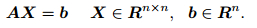
For linear system of equations, A is non-singular matrix and its condition number is calculated as (Li, 2008):

|
(5) |
The linear system of equations is ill-posed when the condition number of A is much greater than 1, cond (A) ≫ 1. The greater the A's condition number is the more ill-posed the linear equation group will be. The solution deviation will be greater by the conventional method (Li, 2008; Xiao, 2003). This study applies formula cond (A)∞ to calculate condition number of linear equation group coefficient matrix.
3 THE SOLUTION FOR ILL-POSED PROBLEMSMeasuring points arrangement is the key factor that whether the coefficient matrix A is ill-posed or not. Firstly, the measuring points arrangement should be optimized so as to realize high precision monitoring of rock mass activity of the target area. And then the methods of pretreatment and regularization are adopted to solve the still ill-posed problems after optimizing.
3.1 Linear Independent OptimizationTo achieve three-dimension location of the seismic source, more than four measuring points shouldn't be installed on the same horizontal plane, otherwise the z coordinates of these points will be equal. A will be a singular matrix detA=0 and A-1 won't exist, which would lead to non-solution or infinite solution of the equation system. Therefore, detA > 0 should be ensured.
Approximate correlation of the row or column vector of the coefficient matrix A, which means the angle between the vectors is very small, is the direct cause of the ill-posed matrix A. The measuring points should be set at unequal interval in three directions of space and arranged randomly so as to build non-singular coefficient matrix A. Ultimately linear system of equations can be solved by direct method. The formulas ai ≠ qaj and ci ≠ qcj should be satisfied, where ai and aj are row vector, ci and cj are column vector, and q is arbitrary real number. The condition number tends to be positive infinity when two arbitrary rows or columns of the coefficient matrix A are proportional and tend to be overlapped completely.
The condition number of matrix A can be reduced effectively by increasing the installation depth difference among sensors for monitoring a wide enough area under the condition that the sensors plane coordinates (xi, yi) are ascertained.
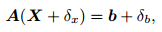
3.2 Initial Coordinates CentralizationThe equations are ill-posed if a small change of the constant term b causes great change of the solution of the equation AX=b. Supposing b is perturbed by value δb, the perturbation of corresponding solution can be calculated as (Liu, 1999):
|
(6) |
|
(7) |
For a certain micro-seismic event, ri, 1, xi, 1, yi, 1 and zi, 1 are fixed values which are determined by the relative position relation of the measuring points, and aren't affected by the points original coordinates value. The right-hand side of formula (4) can be calculated as follows:

|
(8) |
It can be seen from the above formula that the initial coordinate value of x1, y1, z1 has a huge impact on b. If 8 bit integer geodetic coordinates are adopted to indicate x1 and y1, it would cause the huge gap of magnitude order between matrix A and b. Therefore, it needs to transform b to constant term, like A, which wouldn't be affected by initial coordinates, and ensure the solution error will be decreased during regularization solving.
In this study, the following centralization method for the given initial coordinates is put forward.
|
(9) |
|
(10) |
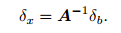
where i=1, …, n. The linear equations are related to the five point coordinates, and therefore only the five xi coordinates participating the calculation are taken into arithmetic mean. The mean value is zero and the variance matrix is invariant after transformation. The same centralized method is used to treat yi and zi, and calculate the right-hand side b with the transformed xi', yi', zi'.
3.3 Row Balance PretreatmentThe difference among xi, 1, yi, 1 and zi, 1 in magnitude order is huge because of the wide monitoring area and simple rapid installation to save cost. Row balance pretreatment to the formula (4) by the following method is proposed so as to reduce the condition number of the coefficient matrix. Non-singular matrix P ∈ Rn×n is selected and the formula (4) is changed into the equivalent equations:
|
(11) |
|
(12) |
|
(13) |
Formula (12) is put forward by Liu (1999), denoted as mmax for short. In this study, the diagonal matrix construction method based on 2-norm is put forward, denoted as m2 as follows:
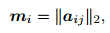
|
(14) |
where ai is the row vector of matrix A, and A=[a1, a2, …, an]T, ‖PA‖2=1. The best construction method would be chosen at the following data processing part by comparing the practical application effect of the two methods.
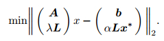
3.4 Regularization InversionA in formula (4) is a bounded linear and compact operator in Euclidean space. The equation has the unique solution when detA ≠ 0. When the condition number is too big, the problem will be unsuitable or ill-posed. To solve this kind of problem, it needs to seek a stable approximate solution in the case of little change in b. The regularized solution xλ (Tikhonov and Arsenin, 1977) is defined as

|
(15) |
where λ is the regularization parameter which controls the weight of relative boundary constraint and the residual norm minimization. L is the boundary limitation matrix. x* is the estimated initial value. Tikhonov method is a direct method, the regularization model is to solve the following least square problem (ELDEN 1977).
|
(16) |
The SVD of A is calculated as follows:
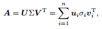
|
(17) |
where ui is row vector in U, vi is row vector in V and i is row index.
The standard form of the Tikhonov regularization model is L=In, x*=0 and the regularized solution is calculated by the following formula (Hansen 2001):
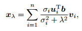
|
(18) |
|
(19) |
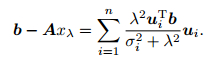
‖xλ‖2 and ‖Axλ -b‖2 play an important role in the judgment of λ. The residual error ‖Axλ -b‖2 will be too large induced by over-regularization of the solution. However, it will be much smaller when there is less regularization of the solution. Nevertheless, the regularized solution will be controlled by data error, which will lead ‖xλ‖2 to be great. L-curve is a compromise curve when two quantities need to be controlled.
Take a set of constants as λ, and substitute them into formula (18) and (19) to solve xλ and b -Axλ. L-curve constitutes x coordinate ‖Axλ -b‖2 and y coordinate ‖xλ‖2 as shown in Fig. 2.

|
Fig. 2 The L-curve |
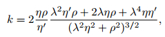
L-curve criterion means the regularization parameter corresponding to the maximum curvature at the L corner is the optimal regularization parameter. The exact optimal regularization parameter can't be obtained directly from the graph. The optimal regularization parameter in Fig. 2 is 0.039833 and its exact numerical solving formula is defined as (Hansen and O'Leary, 2001):
|
(20) |
|
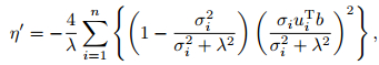
(21) |
where k is the curvature of L-curve. k is regarded as the vertical coordinate and λ is regarded as the horizontal coordinate in Fig. 2. The λ corresponding to curvature maximum value is the optimal parameter.
3.6 Processing Procedure of Ill-posed ProblemsTo avoid ill-posed problems from the beginning, the linear independent optimization should be done in the stage of measuring point arrangement. The available points will be decreased as the working face advancing. Pretreatment and regularization are necessary when the coefficient matrix composed of the remaining points or the optimized points inevitably become ill-posed problems. The specific data processing steps are as follows:
(1) Select the minimum first arrival time point as the base reference, and select another 4 points to form Eq.(4).
(2) To calculate the coefficient matrix A, and solve cond (A)∞. If cond (A)∞ < 10, then skip to step 4. If cond (A)∞≥10, skip to step 3.
(3) Implement centralization and row balance pretreatment.
(4) Implement regularization treatment, and obtain the regularized approximate solution.
4 FIELD TESTING 4.1 Measuring Points ArrangementA certain mine has extremely thick coal seam and its mining method is fully mechanized top caving. For the sake of timely monitoring rock burst to predict mining dynamic hazard, the micro-seismic monitoring system is installed, with eleven triaxial sensors installed in roof and the floor of the track transportation tunnel, as shown in Fig. 3. The black filled dots represent the sensors installed in roof and the squares represent sensors installed in floor. The calibration blasting hole is arranged in the floor.

|
Fig. 3 Monitoring points arrangement graph |
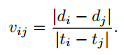
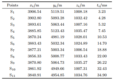
In Table 1, S1, S2, …, S11 are the sensors or measuring points code number, xi, yi, zi are the ith measuring point three-dimensional coordinates, and ti is the first arrival time of P wave. The three-dimensional coordinates of calibration blasting are 3899.89, 5097.48 and 1009.30. S1 is the nearest base point to the source. The two sensors Si and Sj are selected randomly, and the distances between the two sensors to calibration blasting are di and dj. The P wave first arrival time is ti and tj respectively. Therefore, the wave velocity can be calculated by
|
(22) |
|
|
Table 1 Monitoring points coordinates and arrival time |
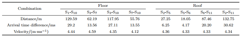
Four groups of floor measuring points combinations and four of top measuring points combinations are selected. The largest interval, the measuring points of crossing the track transportation tunnel, and the smallest interval are gained from the above groups, which can calculate the corresponding velocity vij. The arithmetic mean velocity of all vij is 4.35 m·ms-1, as shown in Table 2.
|
|
Table 2 The wave velocity calculation |
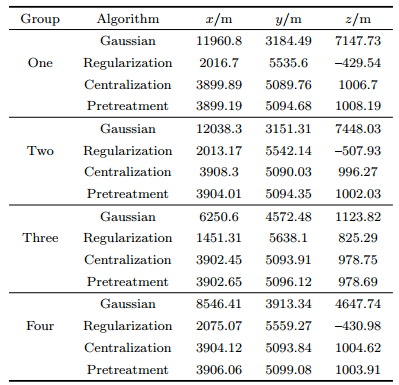
Through designing different inclination angle and different drill hole depth, the three-dimensional direction and differential optimal arrangement is achieved. Unfortunately, it is still limited by the narrow space of the roadway. The maximum distance among z coordinates in bottom is only 1.64 m, and the maximum distance among z coordinates in the roof points is 10.56 m, whereas the maximum distance interval value of y direction measuring points is 174 m. Analysis should be made on the ill-posed problems caused by space layout. The monitoring system layout hasn't gone through linear independent optimization, therefore S1, S3, S7, S10 are almost in the same horizontal plane. When the floor points participate in the seismic source inversion location, there appear severe ill-posed problems in the data of the following 4 groups. Which include combination one (S1, S3, S4, S7, S11), combination two (S1, S3, S9, S10, S11), combination three (S1, S3, S6, S7, S10) and combination four (S1, S4, S7, S9, S11). S1 is the nearest base point to source. The equation solutions are shown in Table 3. Each combination adopts separately the diagonal matrix of m2, mmax structure to balance, and the condition numbers are calculated, as shown in Fig. 3. The calculating methods include Gaussian elimination (Gaussian for short), regularization, regularization after centralization (Centralization for short) and regularization after centralization and row balance (Pretreatment for short). The solution error is shown in Fig. 5.
|
|
Table 3 The optimization processing of four groups data with ill-posed problems |

|
Fig. 4 Condition number of four groups |

|
Fig. 5 Condition number of four groups |
The three kinds of condition numbers of all combinations are basically decreasing as shown in Fig. 4. The condition numbers are largest before row balance pretreatment, and significantly reduced while being calculated with the diagonal matrix constructed by m2. The solution errors calculated by four algorithms are also decreasing, as shown in Fig. 5. The error of Gaussian elimination solution is the biggest, and the source inversion effect by pretreatment and regularization is the best.
In the four combinations, the condition numbers are large without pretreatment, of which the minimum value is 6062.69 and the maximum is 14834.2. Consequently, all of the equations are ill-posed. The minimum of source location error is 2411.34 m and the maximum is 10558.34 m when solved by Gaussian elimination method, and the results aren't significant. The solution error has been improved when Tikhonov regularization algorithm is adopted without pretreatment. The minimum of source location error is 2370.15 m and the maximum is 2514.29 m, nevertheless the error is still great and the data has no applicable value.
By analyzing the characteristics of the initial coefficient matrix A and b, it can be found that the absolute value of the element in A is 102 and the absolute value of the element in b is 106. The initial analysis is that large difference of the order of magnitude causes the great solution error. The four groups data is processed by the centralization pretreatment, and the matrix A has no change therefore the condition numbers haven't decreased. The order of magnitude of righthand side b decreases significantly, and the absolute value of maximum order of magnitude of element is 104, and most of them are 103. If the data after centralization is calculated with Gaussian, the location error can't be improved. However, the location result is greatly improved when Tikhonov regularization method is adopted, and the error of combination one and four is reduced to less than 10 m, the minimum location error is only 7.28 m and the average value is 14.4 m. The results have reached the level of practical application.
After centralization pretreatment, row balance is also used to analyze the data of the four groups, it turns out that cond (A)∞ is improved significantly, and the maximum value is down from 14834.2 to 10818. As is shown in Fig. 4, the condition numbers are calculated with m2 and are smaller than that calculated with mmax in combination one, two and four. Therefore, diagonal matrix constructed with 2-norm, which is put forward in this study to execute row balance pretreatment, has a better effect. Nevertheless, the equations are still ill-posed and should be regularized. The regularized solution after pretreatment is improved significantly in combination one and two. Combination one has the smallest error of 3.09 m, and the error decreases by 0.1 m in combination three. Only in combination four, the error increases by 1.06 m. The location precision is further improved compared to regularization after centralization, and the average error is decreased to 11.6 m. The measuring points arrangement, signal quality, average velocity and etc will influence the solution error.
5 CONCLUSIONSLinear independent optimization is needed in measuring point arrangement when linear method is adopted to invert for seismic source. Four or more than four measuring points shouldn't be set on the same horizontal plane, and the measuring point should be set at unequal interval in three dimensional direction and be arranged randomly. The installation depth difference among sensors should be increased.
The initial value of the measuring points is the most important factor that affects the error level of the source location. The centralization pretreatment is proposed based on the characteristics of the micro-seismic data. The order of magnitude of constant term b decreased greatly while coefficient matrix A isn't affected, and the location error is reduced considerably. The results don't have any significance before centralization, whereas the location results reach the level of practical application after centralization.
The 2-norm of the matrix A's row vector is proposed to construct the diagonal matrix P and impose row balance pretreatment. The condition number of matrix A is decreased effectively, nevertheless, the improvement is limited. It is necessary to implement regularization processing when the equations are heavily ill-posed and can't reach the optimization expectation.
The location error is still large, in case the micro-seismic monitoring data solutions are solved directly. The method of pretreating the data before regularization can greatly improve the solution precision. The minimum location error is 3.09 m. There are three groups of source location inversion error that is less than 10 m. The result reaches the requirement of actual engineering application.
In general, the basis to obtain high precision source solution is optimal arrangement of measuring points, high quality sampling signal, velocity model optimization, etc. In this paper, the available and useful information is extracted from the invalid data that is unable to be processed by conventional method. In the case that the valid signal is monitored by limited points, the accurate source location can also be obtained. This paper provides a new algorithm to solve the ill-posed problems of micro-seismic source location, which promotes the development of the micro-seismic monitoring technology.
ACKNOWLEDGMENTSThe research presented in this paper is supported by Natural Science Foundation of China (51574250), the national key research and development program (2016YFC0801405), and the Science and Technology Development Plan of Shandong Province (2014GSF120017).
| [] | Dong L J, Li X B, Tang L Z, et al. 2011. Mathematical functions and parameters for microseismic source location without pre-measuring speed. Chinese Journal of Rock Mechanics and Engineering (in Chinese) , 30 (10) : 2057-2067. |
| [] | Eldén L. 1977. Algorithms for the regularization of ill-conditioned least squares problems. BIT Numerical Mathematics , 17 (2) : 134-145. DOI:10.1007/BF01932285 |
| [] | Hansen P C, O'Leary D P. 1993. The use of the L-curve in the regularization of discrete ill-posed problems. SIAM J. Sci. Comput. , 14 (6) : 1487-1503. DOI:10.1137/0914086 |
| [] | Hansen P C. 1997. Rank-Deficient and Discrete Ill-Posed Problems:Numerical Aspects of Linear Inversion. Philadelphia:SIAM. |
| [] | Hansen P C. 2001. The L-Curve and Its Use in the Numerical Treatment of Inverse Problems[M]. Southampton: WIT Press . |
| [] | Hansen P C. 2007. Regularization Tools Version 4.0 for Matlab 7.3. Numerical Algorithms , 46 (2) : 189-194. DOI:10.1007/s11075-007-9136-9 |
| [] | Jin M P, Wang R J, Dai S G. 2014. Improvement and case test of linear method for single event seismic location. Acta Seismologica Sinica (in Chinese) , 36 (5) : 757-759. |
| [] | Lawson C L, Hanson R J. 1974. Solving Least Squares Problems. Englewood Cliffs:SIAM. |
| [] | Li Q Y, Wang N C, Yi D Y. 2008. Numerical Analysis. 5th ed. (in Chinese)[M]. Beijing: Tsinghua University Press . |
| [] | Li Y Q, Zhu Y X. 2009. Capsule in vivo environment's TDoA wireless location algorithm and simulation. Microcomputer Information (in Chinese) , 25 (22) : 134-135. |
| [] | Lin F, Li S L, Xue Y L, et al. 2010. Microseismic sources location methods based on different initial values. Chinese Journal of Rock Mechanics and Engineering (in Chinese) , 29 (5) : 996-1002. |
| [] | Liu J G. 1999. Matrix Condition Number and Ill-Posed Improvement[Master thesis] (in Chinese). Chongqing:Chongqing University. |
| [] | Ma C Y, Yang S L, Li S P. 2010. A regularization method of ill-conditioned linear equations. Journal of Gansu Science (in Chinese) , 22 (4) : 33-35. |
| [] | Miller K. 1970. Least squares methods for ill-posed problems with a prescribed bound. SIAM J. Math. Anal. , 1 (1) : 52-74. DOI:10.1137/0501006 |
| [] | Pang H D, Jiang F X, Zhang X M. 2004. Study on nonhomogeneous material's AE by image processing method. Rock and Soil Mechanics (in Chinese) , 25 (Z1) : 60-62. |
| [] | Tian Y, Chen X F. 2002. Review of seismic location study. Progress in Geophysics (in Chinese) , 17 (1) : 147-155. |
| [] | Tikhonov A N, Arsenin V Y. 1977. Solutions of Ill-Posed Problems. Washington:Winston. |
| [] | Wang Y F. 2007. Computational Methods for Inverse Problems and Their Applications (in Chinese)[M]. Beijing: Higher Education Press . |
| [] | Xiao T Y, Yu S G, Wang Y F. 2003. Numerical Solution of Inverse Problem (in Chinese)[M]. Beijing: Science Press . |
| [] | Ye G X, Jiang F X, Yang S H. 2008. Possibility of automatically picking first arrival of microseismic wave by energy eigenvalue method. Chinese J. Geophys. (in Chinese) , 51 (5) : 1574-1581. |
| [] | Zeng X N, Li X H, Jia W M, et al. 2015. A new regularization method for calculating the vertical derivatives of the potential field. Chinese J. Geophys. (in Chinese) , 58 (4) : 1400-1410. DOI:10.6038/cjg20150426 |