 2016, Vol. 59


2 Hunan 5D Geosciences Co., Ltd, Changsha 410025, China
Volcanogenic massive sulfide (VMS) ore deposits on the seafloor are located at mid-ocean ridges, back-arc spreading centers and on volcanoes and seamounts. Some typical hydrothermal areas are known to contain considerable number of sulfide mounds and sulfide ore bodies which have important economic values (Deng X G, 2007; Ьогданов, 2007). At present, the diminishing metallic mineral resources and increasing demand for them have deeply promoted the development of VMS ore deposits prospecting. How to explore the VMS ore deposits in hydrothermal area has become a hot focus.
In recent years, marine transient electromagnetic method (MTEM) used in deep-sea mineral exploration has received extensive attention (Cheesman et al., 1990; Yu et al., 1997; Danielsen et al., 2003; Swidinsky et al., 2015; Börner et al., 2015). Transient electromagnetic response of VMS ore deposits is the basis of applying MTEM to prospect this kind of resource, and some researchers have studied it. Cheesman et al. (1987) calculated the transient electromagnetic response of marine double half-space model to many kind of MTEM configurations. Liu et al. (2006) deduced the TEM response formula of layered model to in-loop configuration and coincident loop configuration through frequency response formula. Swidinsky et al. (2012) produced layered seafloor MTEM response curves for in-loop configuration and coincident loop configuration based on the above study. Zhou et al. (2012) simulated the marine transient electromagnetic response of VMS ore deposit layered model to coincident loop configuration using whole-space theory. Hu et al. (2012) did the 1D forward modeling of TEM response of marine layered model to central loop configuration using cosine transform method. Jang and Kim (2015) studied the one-dimensional forward modeling and inversion of applying an in-loop TEM system to the detection of VMS ore deposits. In the above study, VMS ore deposit was simplified as conductive layer in geophysical model. However, studies of Evans and Everett (1994), Ьогданов (2007), and Swidinsky et al. (2012) on hydrothermal system on Galapagos Ridge, trans-atlantic geotraverse hydrothermal system, and massive sulfide deposits offshore Papua New Guinea show that deep-sea geophysical environment is divided into two half-spaces, sea water and basalt, by the sea-floor, and sulfide ore deposit mounds accumulate on the seafloor with upflow zone and alternation zone below the seafloor as its roots. The entire sulfide ore deposits are three dimensional anomaly body with tapered or lenticular structure in whole space. Xi et al. (2016) simplified the massive sulfide ore deposit as three dimensional target through analyzing the transient electromagnetic response field data of VMS ore deposits collected at the Atlantic mid-ocean ridge and the southwest Indian mid-ocean ridge. So three dimensional forward modeling is the effective way to simulate transient electromagnetic response of VMS ore deposits.
To speed up the calculation and enhance the utility of the algorithm, we simplify the VMS ore deposit as conductive cuboid, and calculate its transient electromagnetic response by full-domain vector finite element method. First, we confirm the validity of our method by comparing our result of a double half-space model to Swidinsky's result. Second, we develop a 3D electrical model of VMS deposit, simulate its TEM response by full-domain vector finite element method, and summarize the characteristics of the response. At last, we validate the numerical simulation result of transient electromagnetic response of VMS ore deposits by physical scale modeling.
2 VECTOR FINITE ELEMENT METHODAs shown in Fig. 1, the electromagnetic boundary conditions of VMS ore deposit, seawater and country rocks are complex. Γin is the boundary of seawater and seafloor, Γa is the border of VMS ore deposit, and Γout is the outer boundary of the computational domain. At these boundaries, the normal component of electrical field is discontinuous while the tangential one is continuous. The conventional node-based finite element method fails to produce accurate results for it requires the continuity of all the electrical field components. Compared to node-based finite element method, vector finite element method produces more accurate results though approximating the whole vector of the electrical field components as one entity (Jin, 2002; Sugeng, 1998; Cai et al., 2014; Huang et al., 2016).

|
Fig. 1 Computational domain σ0 is not considered, σ1=3 S·m-1, σ2=0.01~100 S·m-1, σ3=10 S·m-1. |
Maine transient electromagnetic method is carried out with towed coincident loop configuration, which is only 50 meters above the seafloor (Zhou et al., 2012). Because of the high conductivity of the sea water, the diffusion of the electromagnetic field in the sea water should be considered. Since the VMS deposits are located at mid-ocean ridges and back-arc spreading centers at water depths ranging from 1.5 to 3.7 km, according to the skin depth formula 
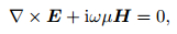
Electromagnetic field can be simulated by solving the Maxwell's equations. Assuming a time harmonic dependence eiωt, the Maxwell's equation in whole space are
|
(1) |
|
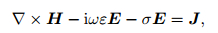
(2) |
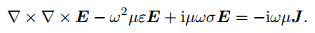
where E is the electrical field, H is the magnetic field, ω is the angular frequency, µ is the magnetic permeability, ε is the dielectric permittivity, σ is the electrical conductivity, and J is the source current density. Taking the curl of Eq.(1), and substituting Eq.(2) into Eq.(1) to eliminate H, we obtained the vector wave equation of electrical field, which is expressed as follows:
|
(3) |
The electrical field in the above equation is total field containing both primary field and secondary field. Since the singularity of the source must be considered in order to solve the total field, the mesh nearby the source must be refined to simulate the quick change of the field, and the unknowns will increase. We solve the secondary field directly. The electrical field in Eq.(3) can be decomposed as
|
(4) |
where Ep is the primary field, and Es is the secondary field. The vector wave equation of the electrical field is decomposed as the following two equations:

|
(5) |

|
(6) |
where ∆σ, the electrical conductivity anomaly, is the difference of the anomaly body conductivity and the background conductivity. The primary electrical field Ep is calculated analytically for a double half-space model. We divide the transmit loop into many electric dipole sources, and calculate the TE mode electrical field of each dipole source (Nabighian, 1987), then integrate it along the transmit loop to solve the primary electrical field.
In deep-sea environment, the conductivity of seawater is 3 S·m-1, the conductivity of basalt is assigned as 0.01 S·m-1, and the sulfide ore deposit has conductivity of 10 S·m-1. Signals with frequencies of 0.1~105 Hz are adopted to transform electromagnetic response in frequency domain to time domain. Since ω2µε ≪ ωµσ is satisfied for the parameters values we assigned, the displacement current can be neglected. Then the secondary electrical field vector wave equation to be solved is reduced to diffusion equation:

|
(7) |
As the computational domain showed in Fig. 1, the secondary electrical field attenuates to 0 on the outer boundary Γout, so a homogenous Dirichlet boundary condition is imposed:

|
(8) |
On the inner boundary Γin and the anomaly body boundary Γa, the tangential component of secondary electrical field is continuous:
|
(9) |
where 
The rectangular brick element we employ to discretize the computational domain is shown in Fig. 2. The numbers indicate the local indices of the edges.

|
Fig. 2 rectangular brick element |
According to the vector basis functions of rectangular brick element, the secondary electrical field within the element can be represented by vector basis function as
|
(10) |
where Eis denotes the tangential component of secondary electrical field along the ith edge. The vector basis functions Ni satisfy the divergence free condition:
|
(11) |
So for the secondary electrical field represented by Eq.(10), we have
|
(12) |
The above equation proves the electrical field presented through vector basis function is divergence free, which guarantees the result is twice differentiable and avoids the spurious solutions. From Eq.(7), the residual of the secondary electrical field can be presented as

|
(13) |
Substituting Eq.(10) into Eq.(13) and using Galerkin procedure (Jin, 2002), the elemental residual Re can be obtained, and its matrix form can be written as
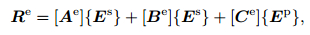
|
(14) |
where [Ae], [Be], [Ce] are 12×12 order elemental matrices defined as follows:
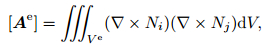
|
(15) |
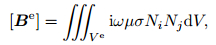
|
(16) |
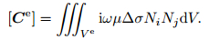
|
(17) |
Assembling elemental Eq.(14) of all the elements, and assigning 0 to the weighted residual of every edge, we obtain equation:

|
(18) |
where K is N × N order global matrix, e corresponds to the unknowns, and b represents the source term. N is the total number of the edges.
For the edges on the outer boundary, assuming its global index is n, the homogenous Dirichlet boundary condition can be imposed by setting

|
(19) |
|
(20) |
Since the vector basis function Ni only has a tangential component along the ith edge, the secondary electrical field presented by Eq.(10) satisfies the continuity condition of tangential component both along element edges and on the element faces.
The secondary electrical field is calculated by solving Eq.(18) with conjugate gradient method. The secondary magnetic field can be calculated by applying Faraday's law to Eq.(10) as
|
(21) |
As the secondary magnetic field Hs is solved, the transient electromagnetic domain response is obtained by converting the frequency domain response through inverse Fourier transform (Kaufman et al. 1987).
3 MODEL CALCULATIONFirst, we examine the accuracy of our algorithm by comparing the result of a double half-space model with Swidinsky's result which was calculated analytically. Then we simplify the VMS ore deposit as a conductive cuboid in double half-space and study its transient electromagnetic response. Our calculations are completed on a personal computer with 2.5 GHz CPU and 4 GB RAM.
3.1 Double Half-Space ModelDouble half-space model of Swidinsky is shown in Fig. 3. The seawater is assigned a conductivity of 3 S·m-1, while the seafloor is assigned conductivities of 1 S·m-1, 3 S·m-1, 10 S·m-1, 30 S·m-1, and 100 S·m-1, respectively.

|
Fig. 3 Double half-space model H-the depth of seawater and seafloor which is infinite. |
Since there is no topography and complex geological structure in the model, we discretize the model with rectangular brick elements and refined the mesh near the seawater-seafloor boundary. The mesh consists of 21×21×14 nodes on each direction respectively, resulting in 6174 nodes and 17493 edges and 5200 elements in total. The computation time is 1459.89, 970.8, 665.69, 279.88, and 211.25 s respectively when the seafloor is of different conductivities. Fig. 4 shows the transient electromagnetic response curve and error, where the symbols represent our results while the lines represent Swidinsky's result. The two results have a good agreement with each other. The maximum error and the average error are 2.97% and 0.31%, respectively, which means our algorithm is accurate.

|
Fig. 4 Transient electromagnetic response curve and error of double half-space model |
A three dimensional electrical model is developed as shown in Fig. 5, in which the VMS ore deposit is simplified as conductive cuboid on the seafloor, and the seawater and basalt are taken as homogenous halfspaces. The seawater and the basalt are given conductivities of 3 S·m-1 and 0.01 S·m-1 respectively, while the VMS deposit is assigned a conductivity of 10 S·m-1. The electrical model shown in Fig. 5 has a regular structure, so it is discretized by rectangular brick elements. The mesh near anomaly body boundary and seafloor boundary is refined, as shown in Fig. 6. The red region represents the anomaly body with dimensions of 200 m×200 m×50 m on the seafloor. The computational domain is 2000 m×2000 m×2000 m in the x, y, and z directions, and contains 47×47×46 nodes in each direction after discretization, resulting in 101614 nodes, 298309 edges and 95220 elements. The transmitter coil and receiver coil are 10 m×10 m square loops. The excited current had an amplitude of 10 A and lasted for 400 ms including a 0.2 ms rise-up time and a 0.2 ms turn-off time. There are 9 observation lines along the east-west direction with 50 m spacing, and 9 points on each observation line also with 50 m spacing, The central point on the main line is exactly at the center of the anomaly upper face. There are 81 observation points in total. It took 263586.15 s to calculate the entire 81 points, which means the average time is 3254.15 s.

|
Fig. 5 Three dimensional model |

|
Fig. 6 Discretization graph of three-dimensional model |
The cuboid indicates the VMS deposit which is located on the seafloor with dimensions of 200 m× 200 m ×50 m. The conductivity of the VMS deposit is 10 S·m-1, while the conductivities of seawater and seafloor are 3 S·m-1 and 0.01 S·m-1 respectively.
The transient electromagnetic response multichannel profile of main line is shown in Fig. 7. To analyze the transient electromagnetic response characteristic of VMS ore deposit directly, we also plot 3D transient electromagnetic response graph using different channel data of all 81 points as shown in Fig. 8.

|
Fig. 7 Transient electromagnetic response multichannel profile of main line |

|
Fig. 8 Numerical simulation of 3D transient electromagnetic response (a) -1.45 ms; (b) -37.81 ms; (c) -61.35 ms. |
As Fig. 7 and Fig. 8 show, the response has a low amplitude and is very smooth in the regions that does not contain the anomaly body. Nearby the anomaly body boundary, the response amplitude suddenly increases from the outside to the inside of the anomaly body region to a certain value, resulting in a high response stage. The high response stage has a similar feature to the anomaly body, which is a diagnostic to discriminate VMS ore deposits. Compare the observation data of early, intermediate and late time, it is obvious that the response in early time is highest and reflects the anomaly body most clearly. As time goes on, the signal decays and the shape of it blurs, which makes the form of the anomaly response changes from square to circle. This change is mainly because the electromagnetic signals are mostly from the deeper seafloor and are less interfered by the sulfide ore deposit on the seafloor.
4 PHYSICAL SCALE MODELINGTo confirm the numerical simulation result, we design and implement physical experiment according to electromagnetic physical scale modeling rules (Nabighian, 1987). The instrument is MTEM-08 marine transient electromagnetic system from Hunan 5D Geo-survey & Technical Company, and the transmitter coil and receiver coil are round loops with diameters of 10 cm. The exciting electrical current is bipolar rectangular square wave with a frequency of 6.25 Hz. A 120 cm×120 cm×85 cm sink filled with brine and the ground below are adopted to simulate the whole space. A copper plate with dimensions of 20 cm×20 cm×5 cm was set on the sink bottom to simulate the VMS ore deposit. There is a 5 cm spacing between each observation position and each observation line. The coincident loop is moved on a horizontal plane on the top surface of the aluminum plate. Fig. 9 shows the 3D electromagnetic response of all the observation data at different time. As seen in the figure, even though the data has disturbance caused by noises, its characteristic has the same pattern with the numerical simulation, which illustrates the numerical simulation is right.

|
Fig. 9 Physical scale modeling of 3D transient electromagnetic response (a) -0.0016 ms; (b) -0.0096 ms; (c) -0.173 ms. |
(1) We use the whole space three dimensional vector finite element method, which discretizes the model with brick rectangular elements, and deduce the finite element equation by employing Galerkin procedure, and convert the frequency domain response through inverse Fourier transform to obtain the time domain response. The method can simulate the transient electromagnetic response of VMS ore deposit effectively.
(2) The comparison between the numerical simulation and the analytical solutions of double half-spaces model and the physical scale modeling result suggests that it is feasible to solve whole space electromagnetic problem using vector finite element method.
(3) For the complex electromagnetic boundary of seawater, ore body and wall rocks, the transient electromagnetic response of VMS ore deposits calculated by whole space vector finite element method has the same features with the physical scale modeling result, and the method is simple, and its results are precise with obvious and clear anomaly response.
ACKNOWLEDGMENTSThis work was supported by the Ocean Major during “Twelfth Five Year Plan” (DY125-11-R-03); the Future Industry Development Special Foundation of Shenzhen (HYZDFC20140801010002); the Marine Development Special Foundation of Hainan (2015XH07).
| [] | Börner J H, Bär M, Spitzer K. 2015. Electromagnetic methods for exploration and monitoring of enhanced geothermal systems-A virtual experiment. Geothermics , 55 : 78-87. DOI:10.1016/j.geothermics.2015.01.011 |
| [] | Cai H Z, Xiong B, Han M R, et al. 2014. 3D controlled-source electromagnetic modeling in anisotropic medium using edge-based finite element method. Comput. Geosci. , 73 : 164-176. DOI:10.1016/j.cageo.2014.09.008 |
| [] | Cheesman S J, Edwards R N, Chave A D. 1987. On the theory of sea-floor conductivity mapping using transient electromagnetic systems. Geophysics , 52 (2) : 204-217. DOI:10.1190/1.1442296 |
| [] | Cheesman S J, Edwards R N, Law L K. 1990. A test of a short-baseline sea-floor transient electromagnetic system. Geophys. J. Int. , 103 (2) : 431-437. DOI:10.1111/j.1365-246X.1990.tb01782.x |
| [] | Danielsen J E, Anken E, Jørgensen F, et al. 2003. The application of the transient electromagnetic method in hydrogeophysical surveys. J. Appl. Geophys. , 53 (4) : 181-198. DOI:10.1016/j.jappgeo.2003.08.004 |
| [] | Deng X G. 2007. The deposits and mineral compositions of hydrothermal sulphides in mid-ocean ridge. Geological Research of South China Sea (in Chinese) (1) : 54-64. |
| [] | Evans R L, Everett M E. 1994. Discrimination of hydrothermal mound structures using transient electromagnetic methods. Geophys. Res. Lett. , 21 (6) : 501-504. DOI:10.1029/94GL00418 |
| [] | Herzig P M, Hannington M D. 1995. Polymetallic massive sulfides at the modern seafloor a review. Ore Geology Reviews , 10 (2) : 95-115. DOI:10.1016/0169-1368(95)00009-7 |
| [] | Hu J H, Chang Y J, Lei S L, et al. 2013. 1D forward of TEM of central loop configuration on sea floor and calculation of all-time apparent resistivity. Geophysical and Geochemical Exploration (in Chinese) , 37 (6) : 1137-1140. DOI:10.11720/j.issn.1000-8919.2013.6.33 |
| [] | Huang W, Yin C C, Ben F, et al. 2016. 3D forward modeling for frequency AEM by vector finite element. Earth Science (in Chinese) , 41 (2) : 331-342. DOI:10.3799/dqkx.2016.025 |
| [] | Jane H, Kim H J. 2015. Mapping deep-sea hydrothermal deposits with an in-loop transient electromagnetic method:Insights from 1D forward and inverse modeling. J. Appl. Geophys. , 123 : 170-176. DOI:10.1016/j.jappgeo.2015.10.003 |
| [] | Jin J M. 2002. The Finite Element Method in Electromagnetics[M]. New York: Wiley-IEEE Press: 93 -113. |
| [] | Kaufman A A, Keller G V. 1987. Frequency and Transient Soundings (in Chinese). Wang J M Trans. Beijing:Geological Publishing House, 257-273. |
| [] | Liu C S, Lin J. 2006. Transient electromagnetic response modeling of magnetic source on seafloor and the analysis of seawater effect. Chinese J. Geophys. (in Chinese) , 49 (6) : 1891-1898. |
| [] | Nabighian M N. 1987. Electromagnetic Methods in Applied Geophysics:Theory[M]. Tulsa, OK: Society of Exploration Geophysicists: 175 -177. |
| [] | Sugeng F. 1998. Modeling the 3D TDEM response using the 3D full-domain finite-element method based on the hexahedral edge-element technique. Exploration Geophysics , 29 (3-4) : 615-619. |
| [] | Swidinsky A, Hlz S, Jegen M. 2012. On mapping seafloor mineral deposits with central loop transient electromagnetics. Geophysics , 77 (3) : E171-E184. DOI:10.1190/geo2011-0242.1 |
| [] | Swidinsky A, Hlz S, Jegen M. 2015. Rapid resistivity imaging for marine controlled-source electromagnetic surveys with two transmitter polarizations:An application to the North Alex mud volcano, West Nile Delta. Geophysics , 80 (2) : E97-E110. DOI:10.1190/geo2014-0015.1 |
| [] | Xi Z Z, Li R X, Song G, et al. 2016. Electrical structure of sea-floor hydrothermal sulfide deposits. Earth Science (in Chinese) , 41 (8) : 1395-1401. DOI:10.3799/dqkx.2016.110 |
| [] | Yu L, Evans R L, Edwards R N. 1997. Transient electromagnetic responses in seafloor with triaxial anisotropy. Geophys. J. Int. , 129 (2) : 292-304. DOI:10.1111/j.1365-246X.1997.tb01582.x |
| [] | Zhou S, Xi Z Z, Song G, et al. 2012. Responses of the towed transient electromagnetic sounding on deep seafloor. Journal of Central South University (Sicence and Technology) (in Chinese) , 43 (2) : 605-610. |
| [] | Ьогданов Ю A. 1994. Modern Ocean sulfide deposits category. Chen B Y Trans. Marine Geology (in Chinese), (4):18-30. |