 2016, Vol. 59


The acquisition of underground velocity distribution by seismic data is a classical problem in seismic exploration, and it is also a difficult problem in the theoretical research of seismic data inversion. There is a nonlinear functional relationship between the seismic wave field and the underground velocity model, and the determination of subsurface velocity model using observed seismic wave field is a typical nonlinear inversion problem. For solving the nonlinear inversion problem, we usually need to give an initial velocity model. From the given velocity model and the source function and the corresponding initial-boundary condition, we can compute the wave field corresponding to the velocity model and obtain the residual wave field between the observed and calculated wave fields. If the residual wavefield is smaller than the threshold, the given velocity model is considered as a subsurface velocity model derived from the seismic wave field. If the residual wavefield is greater than the set threshold, then a correction to the given velocity model is required. According to residual wave field information, the initial velocity model is modified by two main methods: 1) nonlinear optimization method; 2) linear iterative inversion method. The nonlinear optimization method of the first kind includes global optimization method and local optimization method. Due to the huge computational cost of wave field calculation, the local optimization method is usually used to modify the velocity model, which the presently widely studied and used full waveform inversion method. The full waveform inversion method based on local optimization method was proposed in the early 80s of last century (Lailly, 1983; Tarantola, 1984, 1986, 1987), since then it has been the research focus of seismic wave field inversion and has gradually become the underground velocity modeling method in seismic exploration. In this paper, the full-wave inversion based on the local optimization method is called conventional full-waveform inversion. The linearized iterative inversion method of the second type of full-wave inversion is based on the scattering theory of seismic wave propagation (Chew, 1990). Utilizing the asymptotic expansion method (e.g., Taylor expansion, first-order Born approximation, Raytov approximation) the nonlinear full-wave inversion problem is linearized to an iterative linear inversion problem, that is, iterative linear method is used to solve the initial velocity model. Fullwaveform inversion based on local optimization is equivalent to full-waveform inversion based on linearized iterative inversion under the least-squares criterion for data fitting (Vogel, 2002).
The conventional full-waveform inversion has a strong dependence on the initial velocity model, which is the inherent limitation of using the local optimization method to solve the nonlinear inversion problem. In order to reduce this dependency, a variety of multi-scale inversion strategy is proposed, such as Bunks et al. proposed a multi-scale time-domain inversion strategy for different subsets of low to high frequency data (Bunks et al., 1995), Pratt et al. proposed a frequency-domain inversion strategy for seismic data from low-frequency to high-frequency (Pratt et al., 1998; Pratt, 1999). Through the analysis of the objective function of the conventional full waveform inversion, it is considered that the objective function has a higher convexity range in the low frequency band than in the high frequency band, the phenomenon of cycle-skipping which is negative in full waveform inversion can be effectively suppressed in the low frequency band, and it is concluded that full-waveform inversion relies less on the initial model when we use low-frequency data (Sirgue, 2006; Sirgue and Pratt, 2004). Based on the above knowledge, it is very important for the researchers to pay attention to the inversion of the initial velocity model in the full waveform inversion by using various kinds of mathematical transform to extract the low frequency information in the seismic data and to use the low frequency information to do full waveform inversion. Shin et al. proposed the Laplace-Fourier domain and the logarithmic domain full wave inversion method (Shin and Cha, 2008, 2009; Shin and Min, 2006; Shin et al., 2007). Donno et al. proposed normalized integral full waveform inversion method (Chauris et al., 2012; Donno et al., 2013). Bozdaǧ and other researchers proposed envelope full-waveform inversion method (Bozdaǧ et al., 2011; Wu et al., 2014; Chi et al., 2013; 2014). These inversion methods extract the low-frequency information from the seismic data through the mathematical transformation of the data to invert the long-wavelength components of the velocity model. Although these methods have achieved certain results in full-wave inversion, the methods used to extract low-frequency information mostly come from signal transformations, which are not directly related to the mathematical equations describing seismic wave field propagation. Therefore, the mathematical physics of low frequency information is ambiguous.
Conventional full-waveform inversion method considers only the non-linear relationship between seismic wave field and underground velocity model, but does not consider the physical process of seismic wave field propagation, so conventional full-waveform inversion method can be regarded as a purely computational mathematics method. In the propagation of the seismic wave field, the scattered wave field is the most basic wave field, and others such as reflection and refraction wave field are the degradation of the scattering wave field under high frequency approximation. The physical processes of the seismic scattering wavefield propagation include: 1) the incident wave field excited by the source is propagated in the background velocity model; 2) the interaction between the incident wavefield and velocity perturbation relative to the background velocity produces a scattered wave field, and the interaction between the scattered wave field and the velocity perturbation produces a higher order scattering wave field; 3) The scattered wave field propagates in the background velocity model. If the initial velocity model in the conventional full-wave inversion model is regarded as the background velocity model of the scattering wave field propagation equation in the scattering theory, and the propagation equation of the scattered wave field is linearized, then the generation and propagation of the scattered wave field can provide the research idea for the full waveform inversion of seismic wave field.
Based on the above understanding, according to the scattering theory of scattered wave field propagation equation, the propagation equation of second-order integral scattering wave field is deduced firstly, then the linear iterative inversion method under the first order Born approximation is combined with the propagation process of the scattered wave field, at last the second-order integral scattering wave field based on linearized iterative method is proposed. The second-order time integration of wave-field which is equivalent to a low-pass filter can enhance the existing low-frequency data components. Unlike the Laplace, Laplace-Fourier domain full-waveform inversion method, the normalized integral method and the envelope inversion method, the lowfrequency information in seismic data is extracted by various transformations, the method using second-order integral is derived from the scattering wave field propagation equation, which has a clear mathematical physical meaning. In the second-order integral scattering wavefield full waveform inversion, the initial velocity model in the conventional full waveform inversion is regarded as the background velocity model in the scattering wavefield propagation, The residual wave field between the observed wave field and the calculated wave field synthesized by the initial velocity model is regarded as the scattered wave field generated by the velocity perturbation. Based on the derived second-order integral scattering wavefield propagation equation, the distribution of the underground scattering source is reconstructed from the second-order integral residual wavefield of the surface by using the method of back propagation or concomitant propagation, the distribution of ground incident wave field is obtained by means of the forward propagation of the source wave field. Based on the linear relationship between the scattered wave field and the incident wave field and the velocity disturbance in the second order integral scattering wave field linear equation, the correction to initial velocity model is obtained using the imaging formula similar to that used in migration. Finally, the results of the inversion of the secondorder integral scattering wavefield are used as the initial velocity model of the conventional full-wave inversion. The correctness and validity of the full waveform inversion method proposed in this paper are verified by the numerical experiments of Marmousi using full band synthetic data and low frequency cut syntheyic data.
2 METHODS AND THEORYIt is well known that forward modeling is the basis of inversion, so in this section, firstly we derive the propagation equation of the second-order integral scattering wave field and analyze the meaning of second-order time integral wave field. Secondly, we construct the full waveform inversion method based on second order integral scattering wave field propagation equation.
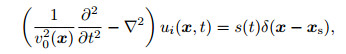
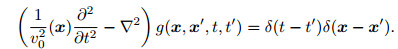
2.1 The Propagation Equation of Second-order Time Integral Scattering Wave FieldIn this paper, the full waveform inversion of single P-wave velocity is considered. Given the initial (background) velocity model and the source function, the propagation equations for the incident wavefield are
|
(1a) |
where xs is the source location, ▽2 is Laplace operator, ▽2=
|
(1b) |
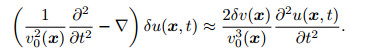
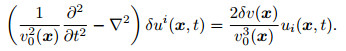
The velocity model is denoted as v(x)=v0(x) + δv(x), δv(x) is velocity perturbation, also known as the correction of the initial velocity model v0(x). According to the scattering theory, the scattering wave field δu(x, t) propagation equation is
|
(2) |
The wave field u(x, t) on the right side of Eq.(2) is the total wave field corresponding to the velocity model v(x). δu(x, t) is known as the perturbation wave field associated with the perturbation velocity model δv(x). Eq.(2) is transformed into the frequency domain by replacing the approximate equal sign in Eq.(2) with an equal sign.
|
(3) |
Set up
|
(4) |
The Eq.(3) can be written as
|
(5a) |
Transform the Eq.(5a) into the time domain
|
(5b) |
According to the expression (4) (the detailed explanation of the formula is in the next section), the wave field δui(x, t) is the second-order time integral of the scattered wave field δu(x, t), we call it the second-order time integral scattering wavefield. Eqs.(5a) and (5b) are frequency domain and time domain forms of the second-order integral scattering wavefield propagation equation, respectively.
The first-order Born approximation is applied in the Eq.(5b):
|
(6) |
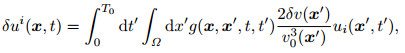
Eq.(6) is second-order time integral scattering wave field δui(x, t) linear propagation equation in first order Born approximation, it is also the basic equations of the full-waveform inversion method. In Eq.(6), there is a linear relationship between velocity perturbation δv(x) and incident wavefield δui(x, t). In order to facilitate the derivation, the Eq.(6) is written in the integral form using the Green function in Eq.(1b):
|
(7) |
T0 is the maximum recording time of the wave field; Ω is the distribution space of velocity perturbation.
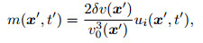
Set up
|
(8) |
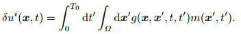
m(x, t) can be regarded as the scattering source of the second-order integral scattering wavefield. It is related to the distribution and strength of δv(x) and ui(x, t). Using Eq.(8), the Eq.(7) can be written as
|
(9) |
The integral in the Eq.(9) is the convolution of the time-space domain. If the left hand of Eq.(9) δui(x, t) is known, it means solving the first kind of Fredholm linear integral equation to obtain the m(x', t'). Make time Fourier transform on both sides of the Eq.(9):
|
(10) |


|
(11) |
We know that the first-order differential operation 


|
(12) |
Integral operation is equivalent to a low-pass filter, therefore, the frequency domain operation represented by Eq.(12) is applied to the wavefield to enhance the low frequency components of the wavefield. Make inverse Fourier transform of Eq.(12):
|
(13) |
F-1 is inverse Fourier transform. Therefore, the low-frequency component of the second-order time integral wavefield u'(t) is enhanced with respect to the original wave field u(t).
The wavefield u(t) is a Ricker wavelet with a dominant frequency of 15 Hz. As shown by the blue line in Fig. 1, the corresponding second-order time integral wavefield ui(t) is shown by the red line in Fig. 1. Their amplitude spectra are shown in Fig. 2. The red line is the amplitude spectrum of Ricker wavelet second-order time integral. As can be seen from the time signal of Fig. 1 and the amplitude spectrum of Fig. 2, the secondorder integral operation enhances the low-frequency components of the Ricker wavelet. The energy of the second-order integral signal is mainly concentrated in the low-frequency band.

|
Fig. 1 The Ricker wavelet with peak-frequency 15 Hz and its second-order time integral: the blue-line denotes Ricker wavelet; the red-line denotes the secondorder time integral of Ricker wavelet |

|
Fig. 2 The amplitude spectrum of Ricker wavelet with peak-frequency 15 Hz and its second-order time integral: the blue-line denotes the amplitude spectra of Ricker wavelet; the red-line denotes the amplitude spectra of second-order time integral of Ricker wavelet |
Figure 3 is the synthetic common-shot gather of Marmousi model, Fig. 4 is the second-order integral wave field obtained by applying second-order integral operation on the seismic wave field in Fig. 3. As can be seen from Figs. 3 and 4, the waveform variation of the wave field in Fig. 4 is slow in comparison with the waveform in Fig. 3. The wave field in Fig. 4 exhibits a significantly lower frequency than the wave field in Fig. 3. Fig. 5 is the envelope of the wave field in Fig. 3. Since the mathematic and physical significance of envelope process and result are not clear. The envelope of signal shown in Fig. 5 is only a non-negative signal whose energy is concentrated in the shallow part and changes very slowly. The second-order integral wave field signal in Fig. 4 is controlled by the wave field propagation equation and is a seismic wave field with definite mathematical and physical significance.

|
Fig. 3 The synthetic common-shot gather of Marmousi model |

|
Fig. 4 The second-order time integral of the synthetic common-shot gather in Fig. 3 |

|
Fig. 5 The envelope of the synthetic common-shot gather in Fig. 3 |
Since the seismic wave field is a nonlinear function of the velocity model, the inversion of the subsurface velocity model v(x) using the observed seismic wavefield data uobs(x, t) is a nonlinear inversion problem. This paper uses the linearized iterative inversion method to solve the problem.
Given an initial velocity model v0(x) and calculate the corresponding synthetic wavefield ucal(x, t), the residual wave field
|
(14) |
As a scattering field caused by a difference in velocity between the subsurface real velocity model and a given velocity model δv(x)=v(x) -v0(x). The second-order integral scattering wave field in the frequency and time domain are calculated.
|
(15) |
|
(16) |
F is the Fourier transform.
According to the propagation equation of the incident wave field and the second-order time integral scattering wavefield linear propagation equation and the Eqs.(8) and (11), we can use δui(x, t) in the time domain or δũi(x, ω) in the frequency domain to retrieve the correction δv(x) for the initial velocity model v0(x). Firstly, we use the known δui(x, t) or δũi(x, t), by solving the linear integral Eq.(9) or (10) to obtain the time domain m(x, t) or frequency domain
|
(17) |
|
(18) |
In the expression, Re represent the real part; symbol * denotes the complex conjugate operation, ui(x, t) and ũi(x, ω) is the time domain and the frequency domain incident ground wave field, respectively. In order to ensure the stability of the calculation, by using the processing method similar to the migration imaging formula, the formula (17) and (18) can be written as
|
(19) |
|
(20) |
After obtaining the solution of the velocity perturbation δv(x), we can modify the initial velocity model v0(x) to get the new velocity model v1(x), that is v1(x)=v0(x) + αδv(x), the α is the modified step size, and then take the v1(x) as the initial velocity model of the next step inversion.
From the above-mentioned inversion step, it is known that the second-order time integral scattering wave field (9) or the linear integral Eq.(10) are the key to solve the time domain m(x, t) or frequency domain
|
(21) |
The least squares solution of the operator Eq.(21) is obtained by using the least squares method
|
(22) |
In the formula, the least squares inverse operator G-1 of the scattering wave field propagator G is given by
|
(23) |
The operation represented by Eq.(22) is the wave-field δui back-propagation in the time-space domain. Because this inverse propagation not only need great computation, but also very unstable, as usual the adjoint operator Gt is used instead of the inverse operator G-1, i.e.,

|
(24) |
The operation represented by Eq.(24) is the propagation of the wavefield in the time-space domain using adjoint (inverse) propagation. This adjoint propagation calculation is small and stable.
Substituting Eq.(23) into Eq.(22), then substitute the Eq.(22) into Eq.(17) to obtain the solution of velocity perturbation estimation, and the inversion results of each common shot set data are superimposed
|
(25a) |
We can also substitute the Eq.(23) into Eq.(22), then substitute the Eq.(22) into Eq.(19) to obtain the solution of velocity perturbation estimation, and the inversion results of each common shot set data are superimposed
|
(25b) |
Substituting Eq.(24) into Eq.(19), we also superimpose the inversion results of each common shot gather data,
|
(26) |
In the above formula, the position of the shot point of the common shot gather is shown by xs; it represents the source wave field propagating forward in the initial velocity model. Eqs.(25a), (25b) and (26) are formulas for solving δv(x) in the time domain.
The above-mentioned time-domain inversion work can also be implemented in the frequency domain, the Eq.(10) in the frequency domain is written as an operator,

|
(27) |
The least squares solution of the operator Eq.(27) can also be obtained by using the least squares method
|
(28) |
In the formula, the least squares inverse operator of the scattering wave field propagator 
|
(29) |
The operation represented by Eq.(28) is the inverse propagation of the wavefield δũi in the frequency-space domain. Similarly, since this inverse propagation is not only computationally expensive, but also very unstable, commonly we use adjoint operator
|
(30) |
The operation represented by Eq.(30) is the propagation of the wavefield in the frequency-space domain with (inverse) propagation. This concomitant propagation is not only computationally small, but also stable.
Substituting Eq.(29) into Eq.(28), (28) is substituted into Eq.(18) to obtain the solution of velocity perturbation, and the inversion results of each common shot gather data are superimposed.
|
(31a) |
Substituting Eq.(29) into Eq.(28), then substitute Eq.(28) into Eq.(20) to obtain the solution of velocity perturbation estimation, and the inversion results of each common shot gather data are superimposed.
|
(31b) |
Substituting Eq.(30) into Eq.(20), we also superimpose the inversion results of each common shot gather data,
|
(32) |
In the above equation, the source wavefield ũi(xs, x, ω) propagating in the background velocity model is represented. Eqs.(31a), (31b) and (32) are formulas for solving δv(x) in the frequency domain.
Substituting the specific form of the forward propagation of the source wave field and the second-order time integral wave field inverse propagation into the Eqs.(31a), (31b) respectively.
|
(33a) |
|
(33b) |
The specific form of the forward propagating source wave field and the second-order time integral wave field propagating backward is substituted into (32),
|
(34) |
In the above formula 
Second-order time integral inversion method can effectively reduce the dependency on the initial velocity model, and the second-order integral wavefield is obviously low-frequency relative to the original wave field, so the resolution of second-order integral inversion results is limited. In order to make full use of all the information in the seismic data to obtain high-resolution full-waveform inversion results, the time-integrated second-order integral wavefield is obtained. The inversion results obtained by the second-order time integral full waveform inversion are used as the initial velocity model of conventional full waveform inversion, and then the conventional full waveform inversion is carried out.
3 NUMERICAL EXPERIMENTIn order to verify the correctness and effectiveness of the proposed second-order time integral wavefield full-wave inversion (IntI), we use the synthetic seismic data of Marmousi model to test. The meshing parameters of the Marmousi model are nx=369, nz=125, dx=25 m and dz=24 m. Fig. 6 shows the velocity distribution of the Marmousi model. The synthetic seismic data has 92 shots, the spacing of shot is 100 meters, there are 369 receivers in each shot, the receiver spacing is 25 meters. Time sampling length is 5 seconds, sampling interval is 2 ms. The source is a Ricker wavelet with a dominant frequency of 8 Hz. Two sets of seismic data are used for the test, one for the full-band seismic data, and the other for the seismic data with frequencies below 4 Hz removed. Fig. 7 shows the initial model.

|
Fig. 6 The velocity distribution of Marmousi model |

|
Fig. 7 The initial velocity model with constant gradient for inversions |
For the synthetic full-wave seismic data full-wave inversion test, we first use the constant gradient velocity model shown in Fig. 7 as the initial velocity model of the second-order integral wavefield inversion, and the time domain formula (26) is used to calculate the speed correction. Fig. 8 shows the inversion results obtained from the full-wave inversion of the second-order time integral wavefield. Compared with Fig. 6 and Fig. 8, the velocity model obtained from the second-order time integral wavefield is correct, but the resolution is low. The velocity model shown in Fig. 8 is taken as the initial velocity model of conventional full waveform inversion (FWI), and Fig. 9 is the result of conventional full-waveform inversion using Fig. 8 as the initial velocity model. For comparison, we also use the constant gradient velocity model shown in Fig. 7 as the initial velocity model for the conventional full waveform inversion, and Fig. 10 is the result of the conventional full waveform inversion using Fig. 7 as the initial velocity model. Comparing Fig. 6, Fig. 9 and Fig. 10, it can be seen that for the same constant gradient initial velocity model, the inversion results of the second-order integral wavefield fullwaveform inversion plus conventional full-waveform inversion (IntI+FWI) are obviously superior to the conventional full-waveform inversion results. For a closer comparison of the details of the two inversion results, Fig. 11 shows the velocity versus depth curves of the two inversion results for the 85235 grid point in the Marmousi model, where the green line is the true velocity and the black line is the initial velocity and the red line is the result of the conventional full waveform inversion, and the blue line is the result of the full-waveform inversion of the second-order time integral wavefield plus the conventional full-waveform inversion. From the velocity-depth curve in Fig. 11, it can be seen that the time-integrated second-order integral wavefield full-waveform inversion combined with conventional fullwaveform inversion can well reconstruct the real velocity model.

|
Fig. 8 The inversion result by full waveform inversion of the second-order time integral wavefield |

|
Fig. 9 The inversion result by full waveform inversion of the second-order time integral wavefield plus conventional full waveform inversion |

|
Fig. 10 The inversion result by conventional full waveform inversion |

|
Fig. 11 The Comparisons of velocity-depth curves of the two inversion results at 85th grid-point and 235th grid-point: the up-panel is for 85th grid-point; the bottom-panel is for 235th grid-point. The green line denotes the true velocity, the black line denotes the initial velocity, the red line denotes the velocity from conventional FWI, the blue line denotes the velocity from full waveform inversion of the second-order time integral wavefield plus conventional FWI |
In order to validate the full waveform inversion method proposed in this paper, a complete waveform inversion method is proposed for seismic data with frequency components below 4 Hz removed. In the experiment, we use the constant gradient velocity model shown in Fig. 7 as the initial velocity model for the full-wave inversion of time integral second-order wavefield, and still use time domain formula (26) to calculate the velocity correction. Fig. 12 shows the inversion results obtained by applying the full-wave inversion of the second-order integral wavefield. We then use the velocity model shown in Fig. 12 as the initial velocity model for the conventional full waveform inversion, and Fig. 13 shows the conventional full-waveform inversion result using the initial velocity model in Fig. 12. As a comparison, we also use the constant gradient velocity model shown in Fig. 7 as the initial velocity model to perform the conventional full waveform inversion and envelope inversion plus conventional full waveform inversion (EI+FWI) for the seismic data lacking low frequency. Fig. 14 shows the results of conventional full-waveform inversion using Fig. 7 as the initial velocity model. Fig. 15 shows the inversion results of envelope inversion combined with conventional full-waveform inversion which use Fig. 7 as the initial velocity model.

|
Fig. 12 the inversion result by full waveform inversion of the second-order time integral wavefield |

|
Fig. 13 The inversion result by full waveform inversion of the second-order time integral wavefield plus conventional full waveform inversion |

|
Fig. 14 The inversion result by conventional full waveform inversion |

|
Fig. 15 The inversion result by envelope inversion plus conventional full waveform inversion |
In contrast to Figs. 6, 13, 14, and 15, it can be seen that for the same constant gradient initial velocity model, the result of second-order time integral wavefield full-waveform inversion combined with conventional full-waveform inversion is obviously the best, the result of inversion of envelope inversion combined with the conventional full-waveform inversion is nest good, and inversion result of pure conventional full-waveform inversion is worst. In order to compare the details of the three inversion results, Fig. 16 shows the velocity-depth curves of the inversion results of grid point 85 and 235 in the Marmousi model. The green line is the true velocity, the initial velocity is black line, the result of the conventional full-waveform inversion is dark red line, the result of the envelope inversion combined with conventional full-waveform inversion is light red. The blue line is the second-order time integral wavefield full waveform inversion combined with the conventional full waveform inversion. From the velocity-depth curve in Fig. 16, it can be seen that the velocity model can be reconstructed well by using the second-order time integral wavefield full waveform inversion combined with conventional full-waveform inversion for the seismic data lacking low-frequency.

|
Fig. 16 The Comparisons of velocity-depth curves of the three inversion results at 85th grid-point and 235th gridpoint: the up-panel is for 85th grid-point; the bottom-panel is for 235th grid-point. In the figure, the green line denotes the true velocity, the black line denotes the initial velocity, the dark-red line denotes the velocity from conventional FWI, the light-red line denotes the velocity from envelope inversion plus conventional FWI, the blue line denotes the velocity from full waveform inversion of the second-order time integral wavefield plus conventional FWI |
Comparing Fig. 8 with Fig. 12 and Fig. 9 with Fig. 13, we can see that the inversion results of the full-band data and the seismic data lacking low-frequency is basically consistent when using the time integral inversion method, which shows that the time-integrated integral wavefield full-waveform inversion method is effective for the seismic data lacking low frequency. Fig. 17 shows the velocity-depth curves of grid points 85, 235 in Fig. 9 and Fig. 13, where the green line is the true velocity, the black line is the initial velocity and the red line is the inversion result of the seismic data lacking low frequency, and the blue line is the inversion result of full-band seismic data. It can be seen from Fig. 17 that there is no significant difference between the inversion results using the seismic data lacking frequency below 4Hz and full-band data.

|
Fig. 17 The Comparisons of velocity-depth curves of inversion result by full band seismic data and inversion result by seismic data lacking low frequencies at 85th grid-point and 235th grid-point: the up-panel is for 85th grid-point; the bottom-panel is for 235th grid-point. The green line denotes the true velocity, the black line denotes the initial velocity, the red line denotes the velocity from inversion result by seismic data lacking low frequencies, the blue line denotes the velocity from inversion result by full band seismic data |
Based on the fact that full-waveform inversion of low-frequency seismic data is insensitive to the local minimum and cycle-skipping problem, the propagation equation of second-order time integral scattering wave field is deduced from the scattering wave field propagation equation. The linearized second-order integral scattering wave equation is applied to the linearized iterative inversion of the nonlinear inversion problem, combined with the linear relationship between scattering wavefield, incident wavefield and velocity perturbation in second-order integral scattering wavefield linear equation, a second-order time integral wavefield full-waveform inversion method is proposed to derive the distribution of subsurface scattering sources and then solve the velocity perturbation. The second-order integral of the seismic wave field can effectively enhance the existing low-frequency components in the wave field and enhance the effect of the low-frequency information in the inversion of the seismic data. The difference between the two methods is also the advantage of this method. The dependence of the second-order time integral wavefield full-waveform inversion method proposed in this paper on the initial model is weakened. The second-order time integration of the wavefield in this paper is derived from the mathematical physics equations describing the propagation of the scattered wavefields, which is different from the method of data transformation in the methods of envelope full waveform inversion and normalized integral full waveform inversion. The second-order time integral wavefield has a clear mathematical and physical meaning. By combining the time integral method with the conventional full waveform inversion method, it can not only obtain the high resolution inversion result but also play a role in the full waveform inversion when the seismic data lack low-frequencies. The numerical experiments in this paper show that there is no significant difference between the two inversion results obtained by using the second-order time integral wavefield full-waveform inversion method for seismic data lacking low-frequency below 4Hz and full-band data.
ACKNOWLEDGMENTSThis work was supported by the National Natural Science Foundation of China (41074133, 41374001).
| [] | Bozdağ E, Trampert J, Tromp J. 2011. Misfit functions for full waveform inversion based on instantaneous phase and envelope measurements. Geophysical Journal International , 185 (2) : 845-870. DOI:10.1111/gji.2011.185.issue-2 |
| [] | Bunks C, Saleck F M, Zaleski S, et al. 1995. Multiscale seismic waveform inversion. Geophysics , 60 (5) : 1457-1473. DOI:10.1190/1.1443880 |
| [] | Chauris H, Donno D, Calandra H. 2012. Velocity estimation with the normalized integration method.//74th EAGE Conference and Exhibition Incorporating EUROPEC 2012. SPE, EAGE, W020. |
| [] | Chew W C. 1990. Waves and Fields in Inhomogeneous Media[M]. New York: Dover Publications . |
| [] | Chi B, Dong L, Liu Y. 2013. Full waveform inversion based on envelope objective function.//75th EAGE Conference and Exhibition Incorporating SPE EUROPEC 2013. EAGE, TU-P04-09. |
| [] | Chi B X, Dong L G, Liu Y Z. 2014. Full waveform inversion method using envelope objective function without low frequency data. Journal of Applied Geophysics , 109 : 36-46. DOI:10.1016/j.jappgeo.2014.07.010 |
| [] | Donno D, Chauris H, Calandra H. 2013. Estimating the background velocity model with the normalized integration method.//75th EAGE Conference and Exhibition Incorporating SPE EUROPEC 2013. EAGE, Tu-07-04. |
| [] | Lailly P. 1983. The seismic inverse problem as a sequence of before stack migrations.//Conference on Inverse Scattering, Theory and Applications. Philadelphia, PA:Society of Industrial and Applied Mathematics, 206-220. |
| [] | Pratt R G, Shin C, Hicks G J. 1998. Gauss-Newton and full Newton methods in frequency-space seismic waveform inversion. Geophysical Journal International , 133 (2) : 341-362. DOI:10.1046/j.1365-246X.1998.00498.x |
| [] | Pratt R G. 1999. Seismic waveform inversion in the frequency domain, Part Ⅰ:Theory and verification in a physical scale model. Geophysics , 64 (3) : 888-901. DOI:10.1190/1.1444597 |
| [] | Shin C, Min D J. 2006. Waveform inversion using a logarithmic wavefield. Geophysics , 71 (3) : R31-R42. DOI:10.1190/1.2194523 |
| [] | Shin C, Pyun S, Bednar J B. 2007. Comparison of waveform inversion, Part 1:Conventional wavefield vs. logarithmic wavefield. Geophysical Prospecting , 55 (4) : 449-464. DOI:10.1111/gpr.2007.55.issue-4 |
| [] | Shin C, Cha Y H. 2008. Waveform inversion in the Laplace domain. Geophysical Journal International , 173 (3) : 922-931. DOI:10.1111/gji.2008.173.issue-3 |
| [] | Shin C, Cha Y H. 2009. Waveform inversion in the Laplace-Fourier domain. Geophysical Journal International , 177 (3) : 1067-1079. DOI:10.1111/gji.2009.177.issue-3 |
| [] | Sirgue L, Pratt R G. 2004. Efficient waveform inversion and imaging:A strategy for selecting temporal frequencies. Geophysics , 69 (1) : 231-248. DOI:10.1190/1.1649391 |
| [] | Sirgue L. 2006. The importance of low frequency and large offset in waveform inversion.//68th EAGE Conference & Technical Exhibition. SPE, EAGE, A037. |
| [] | Tarantola A. 1984. Inversion of seismic reflection data in the acoustic approximation. Geophysics , 49 (8) : 1259-1266. DOI:10.1190/1.1441754 |
| [] | Tarantola A. 1986. A strategy for nonlinear elastic inversion of seismic reflection data. Geophysics , 51 (10) : 1893-1903. DOI:10.1190/1.1442046 |
| [] | Tarantola A. 1987. Inverse problem theory:Methods for data fitting and model parameter estimation. Amsterdam:Elsevier Science Publ. Co., Inc. |
| [] | Virieux J, Operto S. 2009. An overview of full-waveform inversion in exploration geophysics. Geophysics , 74 (6) : WCC1-WCC6. DOI:10.1190/1.3238367 |
| [] | Vogel C R. 2002. Computational methods for inverse problems. Philadelphia, PA, US:Society for Industrial and Applied Mathematics. |
| [] | Wu R S, Luo J R, Wu B Y. 2014. Seismic envelope inversion and modulation signal model. Geophysics , 79 (3) : WA13-WA24. DOI:10.1190/geo2013-0294.1 |