 2016, Vol. 59


2 Department of Earth, Ocean and Atmospheric Sciences, University of British Columbia, Vancouver, V6T 1Z4, Canada;
3 College of Marine Geosciences, Ocean University of China, Qingdao 266100, China
Controlled-source electromagnetic (CSEM) method in frequency domain has evolved into an established technique for land mineral resources prospecting and offshore hydrocarbon exploration (Constable, 2010 ; Yang and Oldenburg, 2012 ; Hu et al., 2013 ; Grayver et al., 2014 ). As the EM explorations now increasingly occur in complex geological environments, on the one hand, interpretation of CSEM data based on the assumption of simple one-dimensional (1D) or two-dimensional (2D) geology cannot always be reliable (Ledo, 2005 ; Siripunvaraporn et al., 2005 ). On the other hand, an increasing trend is to carry out three-dimensional (3D) CSEM surveys in order to improve the spatial resolution of subsurface conductivity structure. Therefore, the desire for reliable and quantitative interpretation of CSEM data requires efficient and stable 3D forward and inversion algorithms. Considerable efforts have been contributed to developing numerical algorithms concerning 3D inversion of CSEM data that can accurately recover subsurface electrical structure over the last decade (Haber et al., 2007 ; Commer and Newman, 2008 ; Plesix and Mulder, 2008 ; Lin et al., 2012 ; Weng et al., 2012 ; Liu et al., 2013 ; Zhao et al., 2016 ). However, the inversion of 3D CSEM data is still a challenging problem in terms of computational cost and efficiency, especially as data volumes have been growing and the subsurface model becomes more complex.
The efficiency of inverse algorithm is heavily dependent upon the performance of the underlying forward solver. One important step in many 3D modeling schemes including finite difference method (FD), finite volume method (FVM) and finite element method (FEM) is to solve the large linear equation system resulting from discretization. Iterative methods (e.g., Krylov subspace methods) are commonly used as forward solvers because they usually need little memory due to only matrix-vector products storage required and are quite fast for computation of single-source solutions (Saad, 2003 ). However, there are two main issues when using iterative solvers for 3D CSEM problems:(1) The ill-conditioning of linear equation systems arising from discretization of Helmholtz equation can lead to poor behavior of iterative solvers and even divergence in some numerically difficult cases, such as models with large spatial ratio grids.(2) Iterative solvers are very time-consuming for multi-source problems because each CSEM source location demands a separate forward calculation (Commer and Newman, 2008 ). These difficulties inevitably become major impediments when iterative solvers are used for solving multi-source CSEM problems. In contrast, direct methods based on matrix factorization can also be used for forward computation. Compared to iterative methods, direct methods provide several advantages. First, they are less prone to ill-conditioning of the linear system to be solved, making them more robust for highly heterogeneous models or non-uniform grids, thus acquiring more accurate solutions for complex scenarios (Grayver et al., 2012 ). Second, they separate the solving of linear system into an expensive matrix factorization and comparably inexpensive forward-backward substitution steps, which make them more suitable for multi-source CSEM problems (Streich, 2009 ). As the factorization algorithms have been gradually improved (Amestoy et al., 2001, 2006 ; Schenk and Gärtner, 2006 ) and more powerful workstations are widely available, direct methods, which are previously prohibited for 3D forward modeling due to expensive cost in terms of memory and computation time, have been increasingly used for solving CSEM 3D forward modeling (Streich, 2009 ; da Silva et al., 2012 ; Jahandari and Farquharson, 2014 ), as well as inverse problems (Oldenburg et al., 2012 ; Grayver et al., 2013 ; Schwarzbach and Haber, 2013 ).
The methods used for solving the linear equation system in forward modeling have a significant impact on the choice of subsequent optimization techniques. In previous CSEM 3D inversions, most schemes employ Krylov subspace iterative methods as their forward solvers. Gradient-based optimization algorithms, such as non-linear conjugate gradient (NLCG) methods (Commer et al., 2008 ; Weng et al., 2012 ; Liu et al., 2013 ) or quasi-Newton (QN) methods (Plessix et al., 2008 ; Schwarzbach and Haber, 2013 ; Zhao et al., 2016 ), are commonly used because of their minimal requirements in terms of memory storage and computational cost. Because only firstorder derivative information of the objective function is required during the minimization process, NLCG or QN methods usually exhibit linear convergence (Wright and Nocedal, 1999 ), leading to large number of inversion iterations required for solving the problem. When direct methods are employed as forward solvers, because decomposition of new system matrix after each model update is required, the number of factorization is thus proportional to the number of inversion iterations. Therefore, the combination of NLCG or QN approaches with direct forward solvers are unfavourable. On the other hand, Newton or Gauss-Newton methods, which exhibit quadratic or nearly quadratic convergence rate by considering both the first- and second-order derivative information of the objective function (Wright and Nocedal, 1999 ), require much fewer iterations than NLCG or QN to reach convergence. Accordingly, Newton-based inversion schemes are favourable when employing direct methods as forward solvers, even if additional effort is required within each iteration.
In this work, we present an efficient approach to 3D inversion of CSEM data based on Gauss-Newton (GN) optimization in combination with a direct forward solver. We first briefly review the 3D CSEM forward problem formulation, and then describe the inversion scheme in detail, including inverse problem formulation, solving of normal equation, strategy for model update and choice of the regularization parameter. Finally, inversion results on synthetic data for land and marine CSEM configurations show that our inversion scheme has excellent convergence rate and only ten-odd to tens of iterations are needed to reach desired misfit, demonstrating its efficiency and stability.
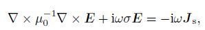
2 THE FORWARD PROBLEMFor CSEM forward modeling problem in the frequency domain, the governing equation that needs to be solved is described by the vector Helmholtz equation for the total electric field E as follows,
|
(1) |
assuming an eiωt time dependence and neglecting displacement currents (i.e., quasi-stationary approximation), where ω is the angular frequency, μ0 is the free space magnetic permeability, σ is the electrical conductivity, and Js denotes applied electric sources. To obtain CSEM responses, a mimetic finite volume (MFV) approximation is employed to discretize Eq.(1). MFV can produce solutions mimicking fundamental properties of their continuum differential operators, thus making the solutions free of spurious modes and physically meaningful (Hyman and Shashkov, 1999a, b ). For orthogonal meshes and isotropic media, MFV method is identical to staggered-grid finite difference method (Smith, 1996 ), but MFV can be naturally extended to non-orthogonal meshes and anisotropic conductivities (Hyman et al., 1997 ; Haber and Ruthotto, 2014 ). For the problem we are concerned here, we only consider orthogonal meshes and isotropic conductivities.
Applying MFV approximation to Eq.(1) on a staggered grid as described in Haber and Rutthotto (2014) , we obtain a linear system for the electric field:

|
(2) |
where A is a complex, sparse and symmetric positive definite matrix, q is the discrete source vector incorporating the electric sources imposed within the model domain and Dirichlet boundary conditions applied on the problem. A direct sparse solver MUMPS (Amestoy et al., 2001 ; 2006) is used to solve Eq.(2). Being a multifrontal solver, MUMPS is efficient in terms of memory and computation time for conducting LU decomposition of non-symmetric matrices or LDLH decomposition of symmetric matrices (Amestoy et al., 2001 ; 2006). For multi-source problems, the system matrix A is invariant at a specific frequency. Therefore, the solutions for multiple source locations can be easily obtained with little additional expense by repeatedly using the same factorization. For detailed investigations on the performance of MUMPS solver, interested readers are referred to Streich (2009) , Oldenburg et al.(2012) and Han et al.(2015) .
3 THE INVERSE PROBLEM 3.1 Formulation of the Inverse ProblemIt is well known that EM data inverse problems are typically non-linear and highly ill-posed. To stabilize the inversion process, we formulate the inverse problem using Tikhonov regularization approach (Tikhonov and Arsenin, 1977 ; Constable et al., 1987 ) as the minimization of the following objective function:

|
(3) |
where β is Tikhonov regularization parameter, and m is the model vector that is parameterized as ln (σ) to enforce a positivity constraint on model parameters. The first term φd (m) is the data misfit that measures the discrepancy between predicted and observed data, which is defined as

|
(4) |
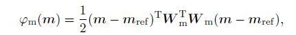
where dobs contains the observed data, Cd is the data covariance matrix characterizing measurement uncertainties, and P is the observation matrix that projects the computed fields at grid points into the measurement locations. While the second term in Eq.(3) is the model regularization term that stabilizes the ill-posed inverse problem, which is defined as
|
(5) |
where mref is the reference model containing a prior knowledge about the model, and Wm is the roughness matrix, having following form (Leliévre and Oldenburg, 2009 ) :

|
(6) |
where Wx, Wy, Wz are first-order finite difference matrices applied to x, y and z directions respectively, and αx, αy, αz are constants that control the roughness of model at different orientations.
In order to obtain the best estimate of the conductivity model that fits the observed data, we employ the Gauss-Newton approach to solve the minimization problem (3). Differentiating the objective function with respect to the model, and set it to zero, we obtain the system of normal equations at each iteration,

|
(7) |
where δm is the model perturbation, g (m) and ${\hat{H}}$ (m) are the gradient and approximate Hessian of objective function, respectively:

|
(8) |

|
(9) |
here J (m) is the sensitivity matrix of CSEM data with respect to model vector m.
3.2 Solving of the System of Normal EquationsTo obtain the model perturbation δm, we need to solve the system of normal Eq.(7) at each GN iteration. Applying implicit differentiation (Rodi and Mackie, 2001 ; Egbert and Kelbert, 2012 ) of Eq.(2) with respect to model parameters m, we obtain

|
(10) |
where u denotes computed fields, and G (m, u) is defined as

|
(11) |
Note that the computation of G (m, u) requires the computed electric or magnetic fields for all source locations and frequencies, which makes the explicit computation and storage of the sensitivity prohibitively expensive for large scale 3D inverse problem. To avoid this, the Eq.(7) is solved by the preconditioned conjugate gradient (PCG) method (Barrett et al., 1994 ) that only requires products of Jocabian and its transpose with vectors for every PCG iteration (Haber et al., 2007 ; Lin et al., 2012 ; Oldenburg et al., 2012 ; Schwarzbach and Haber, 2013 ). Fig. 1 shows the algorithms for matrix-vector products of Jocabian and its transpose with a vector, and detailed description of the algorithms are given in Appendix A. From a computational view, algorithms in Fig. 1 illustrate that the matrix-vector operations of Jocabian or its transpose with vectors are equivalent to one forward or adjoint forward solve, which means two additional forward solves are required at every PCG iteration. When direct solvers are used for the forward modeling, once the system matrix is factored, the factorization can be used repeatedly, and little additional computational effort is needed for PCG iterations.

|
Fig. 1 Algorithms for matrix-vector products of Jocabian and its transpose with a vector |
When the system of normal Eq.(7) is solved iteratively, the PCG system will dominate the inversion process. The exact solutions of Eq.(7) involve substantial computational cost due to the ill-conditioning of the system. An efficient approach to reduce the computation time is to solve Eq.(7) only approximately, which leads to the inexact Gauss-Newton optimization (Nocedal and Wright, 1999 ). The convergence of the inexact Gauss-Newton algorithm is expected as long as the residual of the system of the normal equations is decreasing gradually with PCG iterations (Rieder, 2001 ; 2005 ). Because the inverse problem is highly nonlinear, the inexact solving of Eq.(7) not only reduces the computational cost, but also avoids the oversolving of Eq.(7) at every Gauss-Newton iteration (Eisenstat and Walker, 1996 ), which allows the inversion to escape local minima trapping. In addition, the iterative process in the PCG algorithm has an implicit regularization effect, and the number of PCG iterations controls the magnitude of regularization (van den Doel and Ascher, 2007 ; 2012 ). Typically only ten-odd to tens of PCG iterations are needed to obtain a good model estimate for 3D inverse problem (Oldenburg et al., 2012 ).
An appropriate preconditioner is required to accelerate the solving of Eq.(7). There are mainly two approaches to determine the preconditioner. The first approach is to employ a quasi-Newton algorithm (e.g., L-BFGS) to approximate the Hessian, which is used as the preconditioner (Oldenburg et al., 2012 ). Another approach to precondition Eq.(7) is to utilize the solution of the following linear equation:

|
(12) |
where M can be regarded as the approximate solution to Eq.(7). This approximation is reasonable because the objective function is dominated by the regularization term due to large regularization parameter used at early iterations. Moreover, little additional effort is required to solve equation (12) because of the sparsity of WmT Wm. We have chosen the latter scheme in our implementation to precondition the PCG system at every Gauss-Newton iteration, and the Eq.(12) is solved by the MUMPS direct solver.
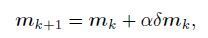
3.3 Model UpdateAfter we obtain the model perturbation δm at each Gauss-Newton iteration, a line search procedure is needed to generate a new model:
|
(13) |
where the step length α is used to control the magnitude of the model update. An accurate seek for the step length α requires solving the univariate optimization problem φ(mk + αδmk) with respect to α, which is too expensive for 3D inverse problem. Instead, we employ an inexact line search strategy to determine a reasonable step length for model update by satisfying the sufficient decrease condition, i.e., the weak Wolfe condition (Nocedal and Wright, 1999 ) :

|
(14) |
where c is a very small constant, here we take 10−4.
3.4 Choice of the Regularization ParameterWe need to specify the regularization parameter β in order to solve the optimization problem in Eq.(3). The regularization parameter β controls the weighting of model regularization relative to data misfit. Therefore, the choice of the regularization parameter has to consider the stabilization of the algorithm and the influence of model regularization to the inverse problem (Siripunvaraporn, 2012 ; Grayver et al., 2013 ). For Tikhonov regularization scheme, the optimal regularization parameter is usually determined by the discrepancy principle between data misfit and model regularization, such as the L-curve criterion. However, this approach entails tremendous computational cost for 3D inverse problem. Instead, we resort to the so called relaxation scheme to determine the appropriate regularization parameter at each iteration (Newman and Alumbaugh, 1997 ; Rodi and Mackie, 2001 ). At early iterations, a large regularization parameter is selected to stabilize the inversion process. Subsequently, the regularization parameter β decreases gradually to put more emphasis on data fitting until a desired data misfit is reached. The regularization parameter βN at each iteration is selected as follows

|
(15) |
where β0 is the initial regularization parameter, is a scalar constant controlling the damping rate of the regularization parameter, and N denotes the current Gauss-Newton iteration.
4 NUMERICAL EXPERIMENTSTo illustrate the efficiency of our CSEM 3D inversion approach, we have considered two synthetic data examples. The first example considers land CSEM data acquisition, while the second example presents synthetic inversion using data from a marine CSEM scenario.
4.1 Land CSEM ExperimentThe model consists of a conductive block of 1 m and a resistive block of 100 m embedded in a homogeneous halfspace of 10 m as shown in Fig. 2. Two anomalous blocks both have dimensions of 1 km×2 km×0.5 km with a depth of burial of 0.5 km. To generate the observed data, the model is discretized with a fine grid of 60×40×40 cells. Besides, to reduce the boundary effects, eight nonuniform padding cells are appended at each side of the model except for the top side, while ten nonuniform cells representing the air layer with a resistivity of 108 m are padded at the top of the model. Thus, the discretization of the computational domain results in 76×56×58 cells in total. The data acquisition consists of 20 transmitter locations with 800 m spacing and 80 receivers with 400 m spacing deployed at the earth's surface. The transmitters are x-oriented horizontal electric dipoles of 100 m length which are excited at 0.25 Hz and 1.0 Hz. By forward modeling, we generate the synthetic data containing x-component of electric fields for transmitterreceiver distance lager than 600 m, and then the synthetic data are contaminated with 3 percent Gaussian random noise resulting in the observed data for inversion.

|
Fig. 2 Planar views of 3D model for land CSEM survey (a) Horizontal slice at z=800 m;(b) Cross-section at y=2000 m. Triangles and circles indicate receivers and transmitters, respectively. |
To test the stability of our inversion algorithm and avoid the so-called inverse crime, we invert the data on a mesh that is different from the one used for forward simulation. The model is discretized into 40×30×40 cells, and the air layer and nonuniform cells are appended onto the model again, resulting in the inversion domain with 52×42×56 cells. The initial regularization parameter β0 and damping factor are set to 0.01 and 2, respectively. The starting model and reference model are the same homogeneous halfspace of 10 m, and the number of PCG is 20 within each GN iteration.
The final inversion results are shown in Fig. 3. From the plan view (Fig. 3a ) and cross section maps (Fig. 3b ), two anomalous blocks are both clearly imaged, although the recovery of the conductive block is better than that of the resistive one, indicating differing resolution of CSEM data with respect to conductive and resistive objects.

|
Fig. 3 Inversion results of land CSEM survey (a) Horizontal slice at z=800 m;(b) cross-section at y=2000 m;(c) 3D view. Cells with resistivity between 5 m and 20 m are cut-off. Triangles and circles indicate receivers and transmitters, respectively. Squares outline the true locations of the anomalous objects. |
Figure 4a shows the convergence rate of GN optimization with iterations. The RMS misfit decreases from 12.78 for the starting model to 1.01 for the final recovered model after nine GN iterations. Besides, Fig. 4b displays a histogram of amplitude ratios between the observed data and predicted data of the initial and final model. It illustrates that the inversion model fit the data from all transmitters and frequencies well, and the final data misfits are within assigned data noise level. Specifically, Fig. 5 shows the data fit distribution for all receivers at the frequency of 1.0 Hz. We can observe that the finial data fitting at almost all receivers is comparably well, and over- or under-fit of data is barely present.

|
Fig. 4 Fitting statistics of 3D inversion (a) Data RMS misfit versus GN iteration for land CSEM survey. The red dashed line shows the desired data misfit at RMS=1;(b) Histogram of the amplitude ratios between observed data used for inversion and predicted data of initial iteration (blue) and of final iteration (red). The red dashed line indicates 3% data error interval. |

|
Fig. 5 (a-c) amplitudes of observed data, (d-f) amplitude ratios between observed data and predicted data of starting model, and (g-i) amplitude ratios between observed data and predicted data of finial model for different transmitter locations with 1Hz transmission frequency for land CSEM survey. Triangles and circles indicate receivers and transmitters, respectively. |
For the second synthetic example, we consider a model modified from 3D SEG/EDGE salt model (Aminzadeh et al., 1997 ) to simulate marine geological environments. The 6 km×6 km×2.8 km model consists of 1 km seawater volume of 0.33 m and a 100 m salt dome object embedded in an uniform background sediment of 1 m shown in Fig. 6. We simulate a realistic 3D marine survey with grid layout illustrated in Fig. 7. The data acquisition geometry comprises twelve orthogonal sail lines with 1 km spacing and thirty-six detectors uniformly deployed on the seafloor with 1 km separation between them. The transmitter is a horizontal electric dipole (HED) placed 50 m above the seafloor, and sends EM signals at 300 m intervals moving along each sail line for three operating frequencies: 0.25, 0.75 and 1.25 Hz. This results in 252 source locations in total.

|
Fig. 6 Planar views of 3D salt dome reservoir for marine CSEM survey (a) XZ section at y=3200 m, (b) Y Z section at x=2000 m. |

|
Fig. 7 Sketch showing data acquisition geometry for marine CSEM survey |
To generate the synthetic data, the computational domain is discretized using a fine grid into 92×92×54 including the air layer and boundary cells as in the case of above land CSEM example. Only inline electric fields parallel to the transmitters orientation are generated. Prior to inversion, five percent Gaussian noise is added to the synthetic data, and a noise floor of 1×10⁻¹⁵ V·m-1(Constable and Weiss, 2006 ) is assumed to decrease the weights of low-amplitude data. Besides, any data point below 5×10¹⁵ V·m-1 are discarded, resulting in 23100 complex data in total. For inversion, the model domain is discretized on a coarse grid into 72×72×46 cells, and the model parameters for inversion is confined to seabed sediments, excluding the air layer and seawater volume. The initial regularization parameter β0 and damping factor are 0.01 and 1.5, respectively. At each GN iteration, 15 PCG iterations are allowed.
A total number of 18 GN iterations are required to reach the target misfit shown in Fig. 8. The RMS misfit decreases from 17.13 for the starting model to 1.07 for the final inversion model, indicating the excellent convergence rate of GN approach.

|
Fig. 8 Data RMS misfit versus GN iteration for marine CSEM survey (The red dashed line shows the desired data misfit at RMS=1) |
Figure 9 displays the inversion results from different cross sections and depth slices. The images clearly resolve the spatial spread of the resistive salt dome, and the maximum value recovered can be as high as 80 m at the core region of the model (Figs. 9h, 9i), demonstrating the excellent resolution of marine CSEM data to resistive targets. Compared to the true model, the recovered resistor is not coincident well with the true salt dome. This is reasonable because the smoothness regularization is expected to smear the images across the discontinuities.

|
Fig. 9 Inversion results shown at different cross sections and depth slices for marine CSEM survey |
The survey consists of thirty-two sea-bottom detectors denoted by red circles and twelve sail lines shown in black lines. The blue curve indicates the projection of the salt dome reservoir at the depth of 1750 m.
5 CONCLUSIONSWe have presented an efficient 3D inversion scheme for CSEM data in the frequency domain, in which the linear system arising from MFV approximation for forward modeling is solved by a direct solver, and the Gauss- Newton algorithm is employed for the minimization. The direct solver used as the forward engine facilitates the reuse of the matrix factorization, which makes the solutions for multiple sources with little additional effort. While the Gauss-Newton approach reduces the tremendous computational cost necessarily associated with the direct solver due to its high convergence rate. By iteratively solving the system of normal equations using preconditioned conjugate gradient method, the need for the explicit computation and storage of the sensitivity matrix is avoided, leading to huge memory savings. These strategies make our inversion approach favourable for 3D CSEM problems.
The first row shows images at different XZ cross sections, the middle row for Y Z sections, and the third row indicates horizontal slices at different depths. The black curve indicates true locations of the salt dome reservoir.
We successfully tested our inversion approach with two synthetic inversion examples for land and marine CSEM surveying configurations. The inversion results from both examples demonstrate the ability and efficiency of our inversion algorithm for multi-frequency and multi-source CSEM problems. With the increasing demand for more accurate imaging of the earth, CSEM surveys in practice are now involving growing number of source locations to improve data coverage. Inversion schemes based on direct forward solvers provide a valuable alternative to current commonly used algorithms based on iterative solvers, although much effort is still needed.
Appendix A Computation of Matrix-Vector Products of Jv and JTwThe Helmholtz Eq.(1) is discretized by MFV using a staggering scheme, resulting in following linear system:

|
(A1) |
where the complex system matrix A is sparse, and symmetric positive definite, e denotes the predicted electric fields at grid points, and q is the discrete source term. To obtain electric fields at measurement locations, we define an observation matrix P of size Nd × Ne, which is independent of model vector m. Here Nd and Ne denote the size of observed data and grid points where electric fields are sampled, respectively. The observed data can be written as

|
(A2) |
and the sensitivity matrix J can be expressed as

|
(A3) |
where Nm denotes the size of model vector m. Applying implicit differentiation to (A1) results in

|
(A4) |
Substituting (A4) into (A3) obtains

|
(A5) |
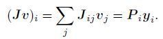
To compute the products of sensitivity matrix J with vector v, defining vector u as

|
(A6) |
and assuming vector y satisfies

|
(A7) |
Combining (A5), (A6) and (A7), we obtain the expression
|
(A8) |
To compute the products of sensitivity matrix transpose JT with vector w, assuming vector z to satisfy

|
(A9) |
Combining (A5) and (A9), we obtain the expression

|
(A10) |
For the total field formulation used in this study, the source term q is assumed to be independent of model vector m, that is, $\frac{\partial q}{\partial m}$ = 0. Due to the symmetry of system matrix A, the computation of (A7) and (A9) are equivalent to one forward and one adjoint solution, respectively.
ACKNOWLEDGMENTSThis work was carried out under the financial support from the National Natural Science Foundation of China (41274077, 41474055), National Basic Research Program of China (2013CB733200), National Science Foundation of Hubei Province (2015CFA019) and China Scholarship Council (201406410020). We acknowledge Eldad Haber and his group at University of British Columbia for many constructive discussions and inspiring suggestions. Detailed comments from three anonymous reviewers have significantly improved the quality of the manuscript.
| [] | Amestoy P R, Duff I S, L'Excellent J Y, et al. 2001. A fully asynchronous multifrontal solver using distributed dynamic scheduling. SIAM Journal on Matrix Analysis and Applications , 23 (1) : 15-41. DOI:10.1137/S0895479899358194 |
| [] | Amestoy P R, Guermouche A, L'Excellent J Y, et al. 2006. Hybrid scheduling for the parallel solution of linear systems. Parallel Computing , 32 (2) : 136-156. DOI:10.1016/j.parco.2005.07.004 |
| [] | Aminzadeh F, Brac J, Kunz T. 1997. 3-D salt and overthrust models. SEG. |
| [] | Barrett R, Berry M, Chan T F, et al. 1994. Templates for the Solution of Linear Systems:Building Blocks for Iterative Methods. 2nd ed. Philadelphia:SIAM. |
| [] | Commer M, Newman G A. 2008. New advances in three-dimensional controlled-source electromagnetic inversion. Geophysical Journal International , 172 (2) : 513-535. DOI:10.1111/gji.2008.172.issue-2 |
| [] | Constable S. 2010. Ten years of marine CSEM for hydrocarbon exploration. Geophysics , 75 (5) : 75A67-75A81. DOI:10.1190/1.3483451 |
| [] | Constable S, Weiss C J. 2006. Mapping thin resistors and hydrocarbons with marine EM methods:Insights from 1D modeling. Geophysics , 71 (2) : G43-G51. DOI:10.1190/1.2187748 |
| [] | Constable S C, Parker R L, Constable C G. 1987. Occam's inversion:A practical algorithm for generating smooth models from electromagnetic sounding data. Geophysics , 52 (3) : 289-300. DOI:10.1190/1.1442303 |
| [] | Egbert G D, Kelbert A. 2012. Computational recipes for electromagnetic inverse problems. Geophysical Journal International , 189 (1) : 251-267. DOI:10.1111/j.1365-246X.2011.05347.x |
| [] | Eisenstat S C, Walker H F. 1996. Choosing the forcing terms in an inexact Newton method. SIAM Journal on Scientific Computing , 17 (1) : 16-32. DOI:10.1137/0917003 |
| [] | Grayver A V, Streich R, Ritter O. 2013. Three-dimensional parallel distributed inversion of CSEM data using a direct forward solver. Geophysical Journal International , 193 (3) : 1432-1446. DOI:10.1093/gji/ggt055 |
| [] | Grayver A V, Streich R, Ritter O. 2014. 3D inversion and resolution analysis of land-based CSEM data from the Ketzin CO2 storage formation. Geophysics , 79 (2) : E101-E114. DOI:10.1190/geo2013-0184.1 |
| [] | Haber E, Oldenburg D W, Shekhtman R. 2007. Inversion of time domain three-dimensional electromagnetic data. Geophysical Journal International , 171 (2) : 550-564. DOI:10.1111/gji.2007.171.issue-2 |
| [] | Haber E, Ruthotto L. 2014. A multiscale finite volume method for Maxwell's equations at low frequencies. Geophysical Journal International , 199 (2) : 1268-1277. DOI:10.1093/gji/ggu268 |
| [] | Han B. 2015. Three-dimensional parallel forward modeling and inversion of frequency-domain CSEM data[Ph.D. thesis](in Chinese). Wuhan:China University of Geosciences. |
| [] | Han B, Hu X Y, Huang Y F, et al. 2015. 3-D frequency-domain CSEM modeling using a parallel direct solver. Chinese J. Geophys , 58 (8) : 2812-2826. DOI:10.6038/cjg20150816 |
| [] | Hu X Y, Peng R H, Wu G J, et al. 2013. Mineral exploration using CSAMT data:Application to Longmen region metallogenic belt, Guangdong Province, China. Geophysics , 78 (3) : B111-B119. DOI:10.1190/geo2012-0115.1 |
| [] | Hyman J, Shashkov M, Steinberg S. 1997. The numerical solution of diffusion problems in strongly heterogeneous nonisotropic materials. Journal of Computational Physics , 132 (1) : 130-148. DOI:10.1006/jcph.1996.5633 |
| [] | Hyman J M, Shashkov M. 1997. Adjoint operators for the natural discretizations of the divergence, gradient and curl on logically rectangular grids. Applied Numerical Mathematics , 25 (4) : 413-442. DOI:10.1016/S0168-9274(97)00097-4 |
| [] | Hyman J M, Shashkov M. 1999a. Mimetic discretizations for Maxwell's equations. Journal of Computational Physics , 151 (2) : 881-909. DOI:10.1006/jcph.1999.6225 |
| [] | Hyman J M, Shashkov M. 1999b. The orthogonal decomposition theorems for mimetic finite difference methods. SIAM Journal on Numerical Analysis , 36 (3) : 788-818. DOI:10.1137/S0036142996314044 |
| [] | Ledo J. 2005. 2-D versus 3-D magnetotelluric data interpretation. Surveys in Geophysics , 26 (5) : 511-543. DOI:10.1007/s10712-005-1757-8 |
| [] | Lelièvre P G, Oldenburg D W. 2009. A comprehensive study of including structural orientation information in geophysical inversions. Geophysical Journal International , 178 (2) : 623-637. DOI:10.1111/gji.2009.178.issue-2 |
| [] | Lin C H, Tan H D, Shu Q, et al. 2012. Three-dimensional conjugate gradient inversion of CSAMT data. Chinese J. Geophys. (in Chinese) , 55 (11) : 3829-3838. DOI:10.6038/j.issn.0001-5733.2012.11.030 |
| [] | Liu Y H, Yin C C. 2013. 3D inversion for frequency-domain HEM data. Chinese J. Geophys. (in Chinese) , 56 (12) : 4278-4287. DOI:10.6038/cjg20131230 |
| [] | Newman G A, Alumbaugh D L. 1997. Three-dimensional massively parallel electromagnetic inversion-I. Theory. Geophysical Journal International , 128 (2) : 345-354. DOI:10.1111/gji.1997.128.issue-2 |
| [] | Nocedal J, Wright S. 1999. Numerical optimization[M]. New York: Springer . |
| [] | Oldenburg D W, Haber E, Shekhtman R. 2013. Three dimensional inversion of multisource time domain electromagnetic data. Geophysics , 78 (1) : E47-E57. DOI:10.1190/geo2012-0131.1 |
| [] | Pidlisecky A, Haber E, Knight R. 2007. RESINVM3D:A 3D resistivity inversion package. Geophysics , 72 (2) : H1-H10. DOI:10.1190/1.2402499 |
| [] | Plessix R é, Mulder W A. 2008. Resistivity imaging with controlled-source electromagnetic data:depth and data weighting. Inverse Problems , 24 (3) : 034012. DOI:10.1088/0266-5611/24/3/034012 |
| [] | Rieder A. 2001. On convergence rates of inexact Newton regularizations. Numerische Mathematik , 88 (2) : 347-365. DOI:10.1007/PL00005448 |
| [] | Rieder A. 2005. Inexact newton regularization using conjugate gradients as inner iteration. SIAM Journal on Numerical Analysis , 43 (2) : 604-622. DOI:10.1137/040604029 |
| [] | Rodi W, Mackie R L. 2001. Nonlinear conjugate gradients algorithm for 2-D magnetotelluric inversion. Geophysics , 66 (1) : 174-187. DOI:10.1190/1.1444893 |
| [] | Saad Y. 2003. Iterative methods for sparse linear systems. Philadelphia:SIAM. |
| [] | Schenk O, Gärtner K. 2006. On fast factorization pivoting methods for sparse symmetric indefinite systems. Electronic Transactions on Numerical Analysis , 23 (1) : 158-179. |
| [] | Schwarzbach C, Haber E. 2013. Finite element based inversion for time-harmonic electromagnetic problems. Geophysical Journal International , 193 (2) : 615-634. DOI:10.1093/gji/ggt006 |
| [] | Siripunvaraporn W. 2012. Three-dimensional magnetotelluric inversion:an introductory guide for developers and users. Surv. Geophys. , 33 (1) : 5-27. DOI:10.1007/s10712-011-9122-6 |
| [] | Siripunvaraporn W, Egbert G, Uyeshima M. 2005. Interpretation of two-dimensional magnetotelluric profile data with three-dimensional inversion:synthetic examples. Geophysical Journal International , 160 (3) : 804-814. DOI:10.1111/gji.2005.160.issue-3 |
| [] | Smith J T. 1996. Conservative modeling of 3-D electromagnetic fields, Part Ⅱ:Biconjugate gradient solution and an accelerator. Geophysics , 61 (5) : 1319-1324. DOI:10.1190/1.1444055 |
| [] | Streich R. 2009. 3D finite-difference frequency-domain modeling of controlled-source electromagnetic data:Direct solution and optimization for high accuracy. Geophysics , 74 (5) : F95-F105. DOI:10.1190/1.3196241 |
| [] | Tikhonov A N, Arsenin V I A K. 1977. Solutions of Ill-Posed Problems. Washington, D. C., USA:W. H. Winston and Sons. |
| [] | van den Doel K, Ascher U M. 2007. Dynamic level set regularization for large distributed parameter estimation problems. Inverse Problems , 23 (3) : 1271-1288. DOI:10.1088/0266-5611/23/3/025 |
| [] | van den Doel K, Ascher U M. 2012. Adaptive and stochastic algorithms for electrical impedance tomography and DC resistivity problems with piecewise constant solutions and many measurements. SIAM Journal on Scientific Computing , 34 (1) : A185-A205. DOI:10.1137/110826692 |
| [] | Weng A H, Li D J, Li Y B, et al. 2015. Selection of parameter types in Controlled Source Electromagnetic Method. Chinese J. Geophys. (in Chinese) , 58 (2) : 697-708. DOI:10.6038/cjg20150230 |
| [] | Weng A H, Liu Y H, Jia D Y, et al. 2012. Three-dimensional controlled source electromagnetic inversion using non-linear conjugate gradients. Chinese J. Geophys. (in Chinese) , 55 (10) : 3506-3515. DOI:10.6038/j.issn.0001-5733.2012.10.034 |
| [] | Yang D K, Oldenburg D W. 2012. Three-dimensional inversion of airborne time-domain electromagnetic data with applications to a porphyry deposit. Geophysics , 77 (2) : B23-B34. DOI:10.1190/geo2011-0194.1 |
| [] | Zhao N, Wang X B, Qin C, et al. 2016. 3D frequency-domain CSEM inversion. Chinese J. Geophys. (in Chinese) , 59 (1) : 330-341. DOI:10.6038/cjg20160128 |