1 INTRODUCTION

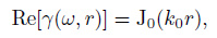
Traditionally, surface wave tomography method for studying the earth structure is based on the data from earthquake events. This method, however, confines the research regions to specific areas because earthquakes occur at specific time and location (Shapiro and Campillo, 2004 ; Sabra et al., 2005a ; Yang et al., 2007). In contrast, ambient noise exists on the earths' surface widely, which is not limited by space and time (Prieto et al., 2011). Utilizing ambient seismic field to study underground structure can overcome the limitation due to the earthquake events. Aki (1957) suggested that for purely elastic media, the azimuth average of spatial autocorrelation γ(ω, r) of the ground motions between two points separated by a distance r could be expressed by a zero-order Bessel function

(1)

where Re[…] denotes taking the real part of the complex argument, ω is the angular frequency, k₀ is the wave number. Employing this relation to investigate the microtremors, phase velocity can be estimated via Eq.(1) and the earth's velocity structure can be studied.

Similar methods based on the continuous seismic noise were put forward in recent years and have achieved great development to study the subsurface structure (Shapiro et al., 2005 ; Zheng et al., 2010 ; Yao et al., 2011 ; Li et al., 2014) since it was proved that the noise cross-correlation function (NCF) recorded at two stations is proportional to the Green's function between these two stations, as indicated by Lobkis and Weaver (2001) based on normal-mode theory. Hence the noise cross-correlation function, which can produce stable empirical Green function mainly corresponding to the surface waves, is used to calculate surface wave phase velocity between stations (Wapenaar et al., 2010a ; Wapenaar et al., 2010b ; Liu and Huang, 2010). Utilizing the information of NCF, many researchers have performed surface wave tomography (Lin et al., 2008 ; Fang et al., 2009 ; Tang et al., 2011 ; Lu et al., 2014 ; Fan et al., 2015).

Most researches focused on the phase information of NCF, i.e. they mainly measure the travel-time of the surface wave in NCF. Recently researchers began to pay attention to the amplitude measurement of NCF (Lin et al., 2011 ; Liu et al., 2013 ; Weemstra et al., 2013 ; Weemstra et al., 2014 ; Liu et al., 2015). Pretio et al.(2009) empirically conjectured that in attenuating medium, after azimuthal averaging, the real part of the normalized cross-correlation (coherency) in frequency-domain is equal to the product of the first kind of zero-order Bessel function with an exponential decaying term

(2)

Using this relation to perform a fitting with observed coherent data, Pretio et al.(2009) calculated the attenuation coefficients for Southern California at period of 5~20 s. However, the introduction of the attenuation term e^{-α(ω) r} in Eq.(2) is a simple extension for elastic medium without the exhaustive and rigorous analysis (Prieto et al., 2009 ; Prieto et al., 2011 ; Lawrence and Prieto, 2011). Therefore, it is difficult to quantify the accuracy of the measured attenuation coefficients because of the lack of necessary theoretical background (Tsai, 2011).

The amplitude of NCF is affected by seismic intrinsic attenuation, noise source distribution and scattering (Lawrence et al., 2013). It is still controversial whether the intrinsic attenuation can be extracted from ambient seismic noise field, which is not uniformly distributed and varies with time and space. Although the azimuth averaging can mitigate the effect of inhomogeneous noise distribution (Prieto et al., 2009 ; Prieto et al., 2011) and time averaging for normalized correlation is able to alleviate directionality of ambient noise source (Lu et al., 2009 ; Tsai and Moschetti, 2010 ; Lawrence et al., 2013). Based on the method of Yokoi and Margaryan (2008), Nakahara (2012) demonstrated that the expression J₀(k₀r) e^{-α(ω) r} only holds approximately for small attenuation. The numerical experiment of Cupillard and Capdeville (2010) indicated that the amplitude strongly depends on the distribution of noise source. Weaver (2011) and Tsai (2011) suggested attenuation coefficients cannot be recovered from azimuth averaged coherency.

In this article, we consider a model that noise source is uniformly distributed at the circumference with a larger radius. Under this distribution, we study the coherency expressions in dissipative media and discuss the potential influence due to different normalized factors. Finally, possible results are analyzed when directly employing the Eq.(2) to compute the attenuation of earth medium.

2 MODEL ASSUMPTION AND COHERENCY DEFINITION

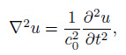
In purely elastic medium, the time-domain wave equation is

(3)

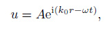
where u is the wave field, c₀ is phase velocity which is always a real number. For a monochromatic wave propagating along a special direction, the solution of the wave equation can be written as

(4)

where A is wave amplitude, wavenumber is given by k₀ = ω/c₀. Accordingly, the wave equation in frequency domain is

(5)

The wave equation in time domain is modified by considering attenuation:

(6)

where α is the attenuation coefficient. Correspondingly in frequency-domain it reads

(7)

That is

(8)

Defining the complex wave number as k= k₀ + iα and substituting it into Eq.(8) yields

(9)

The solution of Eq.(9) is obtained as

(10)

The noise source distribution in this study is shown in Fig. 1. A series of sources are uniformly distributed at a circumference with the radius R. a and b are the locations of two receivers which are respectively expressed as r₁ and r₂. Comparing with |r₁| and |r₂|, the distance between a and b, the radius R can be regarded as infinity, i.e. R→∞. In this case, the wave received at a and b can be seen as the plane wave as shown in Eq.(10). Therefore, the plane waves received at two stations from a single excitation source can be described:

(11)

(12)

Meanwhile, it is assumed that the waves excited by different sources are mutually uncorrelated. They satisfy

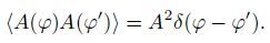
(13)

Wave vector is given by k= k${\hat{k}}$ =(k₀+iα)${\hat{k}}$ = k₀+iα${\hat{k}}$. ${\hat{k}}$ is unit vector in the direction of wave propagation which satisfies ${\hat{k}}$ = -R/|R|. φis the azimuth and represents ensemble average.

For impulsive or transient sources, we generally first calculate the cross-correlation of the field recorded at two points due to the single source and then sum up the results for all sources available. The order of the correlation and summation should not be changed in order to avoid the non-physical cross-terms (Wapenaar et al., 2010a). For the ambient seismic noise, which is the superposition of all sources available, it is difficult to separate the records from different sources. The cross-correlation is always conducted for the summation records of all sources. Fortunately, cross-terms do not appear in NCF since the noise field from different sources is usually unrelated. In this paper, the active multi-sources are considered for the attenuating medium. The order of the summation and cross-correlation is important. Hence two cases are discussed in this study according to the order of summation and cross-correlation: summation-correlation and correlation-summation.

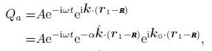
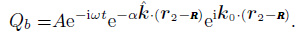
For the case of summation-correlation, as shown in Fig. 1, it was assumed the noise source is located at R, and the fields recorded at r₁ and r₂ are the summation over all sources. The R is large enough so that the field received at stations a and b can be thought as the plane wave, which are respectively expressed by

(14)

(15)

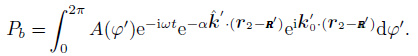
In frequency domain, their correlation is expressed by the multiplication with one of them taken as the complex conjugate

Since the integration variable φ and φ is mutually independent, it can be written as

(16)

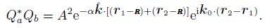
Thanks to Eq.(13), the ensemble average of the correlation function is derived as

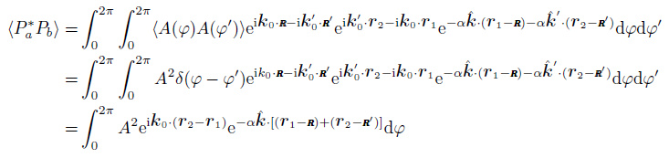
(17)

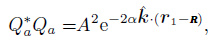
The autocorrelations at respective point are

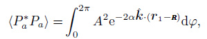
(18)

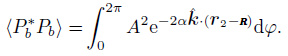
(19)

Spatial coherency has three definitions by taking different normalized factors,

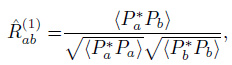
(20)

(21)

(22)

For the case of correlation-summation, according to Eq.(11) and Eq.(12), the correlation function between the receivers a and b is

(23)

The autocorrelation functions at the points a and b can be written as

(24)

(25)

Similarly, three kinds of coherency are defined respectively as

(26)

(27)

(28)

3 SPATIAL COHERENCY EXPRESSIONS IN AN ATTENUATING MEDIUM 3.1 Summation-Correlation

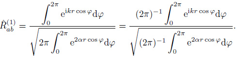
Substituting Eqs.(17), (18) and (19) into Eq.(20) leads to

(29)

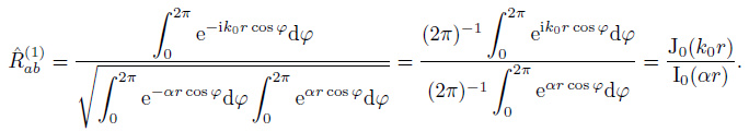
Figure 2 shows a specific coordinate system in which station a is located at the ordinate origin and station b is placed at the positive X-axis with distance r from a. Thus, r₁ = 0, r₂ = r, k₀ · r₂ = -rk₀ cosφ, and ${\hat{k}}$ · r₂ = -r cosφ. Eq.(29) can then be written as

(30)

According to the Eq.(9.1.18) and Eq.(9.6.16) in Abramowitz (1970), the Eq.(27) in Cox (1973), the zero-order Bessel function J₀(z) and the zeroorder modified Bessel function I₀(z) respectively satisfy . Therefore Eq.(30) has a simplified expression

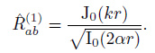
(31)

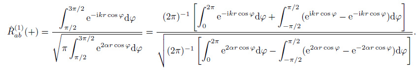
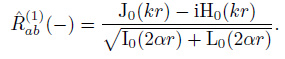
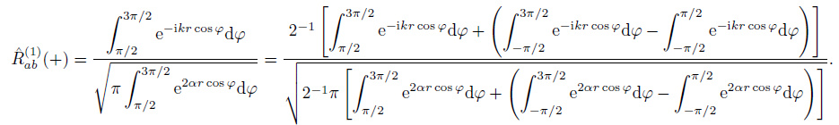
The correlation function in time domain includes the causal and anti-causal part. The casual part represents the wave field propagating from a to b due to the sources located on the one-side semicircle (φ∈[π/2, 3π/2]) close to point a, as shown in Fig. 3. While the anti-causal part represents the wave field propagating from b to a due to the sources located on the other side semicircle (φ∈[-π/2, π/2]). For casual sources, the coherency is given by

(32)

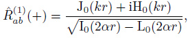
On the basis of the Eq.(12.1.7) and (12.1.7) in Abramowitz (1970), the zero-order Struve function H₀(z) satisfies and the zero-order modified Struve function L₀(z) satisfies 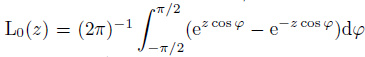. The following relation is then obtained (the details are shown in Appendix A).

(33)

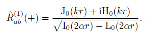
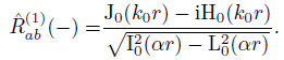
Similarly, for anti-causal sources, the coherency is

(34)

As Weaver (2012) pointed out, Eq.(13) means the wave field is fully isotropic only at the origin. For the coordinate system shown in Fig. 2, only the wave field at point a is fully isotropic. However, if the coordinate origin is taken as the midpoint between a and b, the wave field at point a will not be fully isotropic. Unlike the purely elastic case, in attenuating medium, the expressions of spatial coherency between the two stations will change if we change the location of coordinate origin. As shown in Fig. 4, if the origin is taken as the mid-point between a and b, we have . The coherency expression defined by Eq.(20) would be written as

(35)

Similarly, the coherency for the causal and anti-casual part is then written as

(36)

(37)

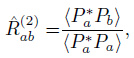
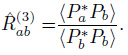
As coherency expression defined by Eq.(21) and (22) with different normalizing factors, they are listed in Table 1 and Table 2, which can be obtained by performing the similar derivation.

Equations (35), (36) in this study are consistent with Eqs.(25)(29) in Tsai (2011) where the similar results were present based on the same noise source models which are called uniform distribution of farfield surface waves and one-side far-field surface waves. Thought it is assumed that noise sources are uniformly distributed at a circumference with large radius R, the wave field at each point inside the circle is not identical if the medium attenuation is taken into account. When the coordinate system shown in Fig. 4 is taken, according to Eq.(13), only the wave field at the midpoint between a and b is isotropic. Considering from the viewpoint of source distribution, two choices of the coordinate origin imply the noise sources have different azimuth distributions with respect to the location a and b. In damping medium, source distribution affects the expression of spatial coherency and using the exponential decaying term of Eq.(2) to recover attenuation coefficients may cause the potential unreliability.

3.2 Correlation-Summation

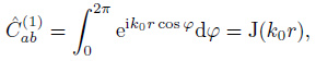
The order of correlation and summation is important for impulsive sources or transient wavelets. In order to avoid the cross-term, we should first correlate the records between a and b for a single excitation source and then sum up all the correlation results due to different sources. For this case, to begin with the first definition in Eq.(26), substituting Eqs.(23), (24) and (25) into Eq.(26) results in

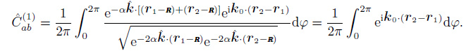
(38)

Similarly, it can be easily derived

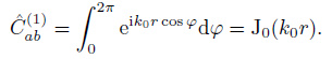
(39)

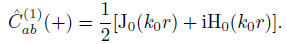
For the causal part, which can be written as

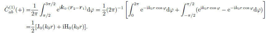
(40)

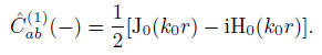
For the anti-causal part, it is

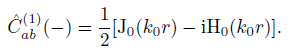
(41)

If we take the mid-point between point a and b as the origin, as shown in Fig. 4, same results can be obtained.

(42)

(43)

(44)

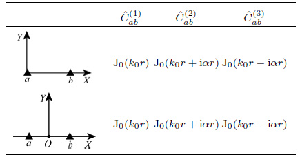
The expressions for Eqs.(27) and (28) can be obtained by similar calculation, which are present in Table 3 and Table 4.

4 ANALYSES AND DISCUSSION

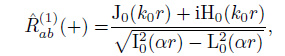
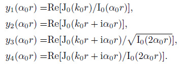
Different coordinate systems are equivalent to different azimuth distributions of noise sources. The results from Table 1 to Table 4 demonstrate the spatial coherency expressions in attenuating medium are dependent on the source distribution. As the ambient seismic noise is concerned, the recorded signals at selected stations have been the superposition of waves from all the sources, we need only discuss the case of summation-correlation when we try to recover attenuation from ambient noise field. As shown in Table 1, in this case, there are 4 kinds of expressions for the real part of coherency due to different selections of normalizing factors, which are renamed as

(45)

Figures 5a -5d respectively present the 4 kinds of coherency as a function of interstation distance k0r for the period T= 7.5 s, the phase velocity c₀ = 3.08 km·s^-1, and the attenuation coefficient α = 0.0024 km^-1. As a comparison, the exponential-decay spatial coherency J₀(k₀r) e^{-α(ω) r} in Prieto (2009) and the coherency J₀(k₀r) of elastic case are also given. For the given attenuation coefficient α and period T, the curve for coherency expression J₀(k₀r) e^{-α(ω) r} given by Prieto (2009) decays most rapidly with the increase of k0r. This indicates that a higher attenuation value α is required in order to make the decline rate of the curves denoted by the other expressions keep up with the exponentially decaying rate expressed by J₀(k₀r) e^{-α(ω) r}. Or, equivalently the attenuation coefficient obtained by fitting the observed data with J₀(k₀r) e^{-α(ω) r} is smaller than the real one. Figs. 5b and 5c demonstrate that the amplitudes for both Re[J₀(k₀r+iαr)] and are even higher than the amplitude of spatial coherency in elastic case. This implies a negative attenuation coefficient is needed to explain it, which is obviously inconsistent with the actual physical reality. Tsai (2011) also found and discussed the similar problem.

Supposing the quality factor does not vary with frequency (Kjartansson, 1979), for the case of weak decay, the relation between attenuation and frequency is

(46)

Taking the values of r= 200 km, Q= 50 and c₀ = 3.08 km·s^-1, different attenuation models could be produced by invoking the relation shown in Eq.(46) and normalizing the spatial coherency expressions in Eq.(45) by J₀(k₀r). Fig. 6 shows the decay curves as a function of the attenuation coefficient. It can be found that the exponentially decaying rate is the fastest. As mentioned previously, for positive attenuation coefficient, the curves of the coherency expressions by do not decrease with an increase of attenuation coefficient. We conjecture that the reason for this particular phenomenon is due to the source distribution. ${\hat{R}}$ _ab ⁽¹⁾ and ${\hat{R}}$ _ab ⁽²⁾ are the outcomes of choosing different normalizing factors and both of them are obtained under the coordinate system described in Fig. 2, where the sources are uniformly distributed along the circumference. The field at each point inside the circle, except the point a, is not isotropic. Therefore it is the specific distributed sources that cause these particular results and the correlation technology is invalid in this case to extract the attenuation.

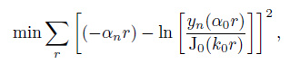
Prieto (2009) studied the attenuation coefficient in southern California by fitting the observed data acquired by NCF with the expression J₀(k₀r) e^{-α(ω) r}. The decay coefficients and phase velocities for 4 typical periods were as follows: T= 7.5 s, c₀ = 3.08 km·s^-1, α = 0.0024 km^-1; T= 10 s, c₀ = 3.15 km·s^-1, α = 0.0019 km^-1; T= 15 s, c₀ = 3.34 km·s^-1, α = 0.0006 km^-1; T= 20 s, c₀ = 3.53 km·s^-1, α = 0.0002 km^-1(Prieto et al., 2009). We take these attenuation coefficients as the actual earth's attenuation coefficients, and denoted by α0, to examine the expressions we give in Eq.(45). Theoretically, for different noise source model α0 satisfies one of the 4 expressions of ${\hat{R}}$_ab shown in Eq.(45). In order to analyze the discrepancies between this theoretical expression with J₀(k₀r) e^{-α(ω) r}, we employ J₀(k₀r) e^{-α(ω) r} to perform least square fitting with 4 expressions (y_n (n = 1, 2, 3, 4)) shown in Eq.(45), i.e. we seek the α_n (n = 1, 2, 3, 4) which minimize the following objective function.

(47)

where ln means natural logarithm. Fig. 7 shows the least-squares solutions of Eq.(47). It is observed that the attenuation coefficients obtained by fitting the curves expressed in Eq.(45) using J₀(k₀r) e^{-α(ω) r} is lower than the real values.

Different spatial coherency expressions are needed for the models with different source distributions. This suggests that these models are not good enough to simulate the ambient noise coherency in the attenuating Earth. As Walker (2012) demonstrated, the attenuation causes the inhomogeneity of plane wave unavoidably. Therefore the spatial coherency varies with normalizing factors and source distributions, which makes the corresponding results dependent on the choice of coordinate systems. This fact indicates it is not perfect to describe the earth's attenuation with the similar model in this study. The earth ambient noise model cannot be simulated fully by the surface wave sources distributed on a 2-D plane and we should consider the volume distribution of noise sources. On the other hand, it reminds us we must be more cautious when utilizing the noise correlation technology to recover the medium attenuation.

5 CONCLUSION

In this study, a model is introduced in which the sources are uniformly distributed along a circle with large radius so the waves can be seen as a plane wave and they are also assumed to be uncorrelated. Based on this model, we derive the spatial coherency expressions between two points inside the circumference and analyze the application of these expressions to extract the attenuation coefficients of medium adopting ambient noise correlation technology. The study suggests the spatial coherency expressions are affected by the source distribution and the expressions are different for different normalizing factors. The present models are not good enough to describe the coherency expressions of the actual attenuating medium in the Earth. The attenuation coefficients recovered by traditional approaches of employing the coherency expression J₀(k₀r) e^{-α(ω) r} may be smaller than the real values.

Appendix A Derivation for Equation (32) and Equation (33)

From the Eq.(29), the coherency expression for the casual sources is given by

(A1)

Taking the properties of periodic function into account, it yields

(A2)

After several simple integral computations, the Eq.(A2) simplifies to

(A3)

Here, the Eq.(A3) is the Eq.(32) in the text.

According to the Eq.(12.1.7) in Abramowitz (1970)

And the Eq.(12.2.2)

Let v = 0, we have

(A4)

(A5)

Finally, substituting Eqs.(A4) and (A5) into Eq.(A3) results in

(A6)

where the Eq.(A6) is the Eq.(33) in the text.

ACKNOWLEDGMENTS

This work was supported by the National Natural Science Foundation of China (41174041).