 2016, Vol. 59


2 China Research Institute of Radiowave Propagation, Qingdao 266107, China
Currently, ground-based instruments for ionospheric detection mainly contain vertical sounders, oblique sounders and backscatter sounders. One can get ionospheric electron density information over the ionosonde station when vertically sounding. In terms of acquiring the height profile of ionization over a single site, vertical sounders are the most direct and accurate among the three types of ionospheric sounding instruments. Oblique sounding can achieve site-to-site ionospheric detection, however, only the ionospheric information from reflection region corresponding to the fixed ground distance can be got using the inversion results. Backscatter sounding is characterized by detecting long distances, covering wide ranges and obtaining large areas of ionospheric parameters and becomes the unique technique to get the state of the ionosphere in remote areas. This is the greatest advantage of backscatter sounding over vertical and oblique soundings. For some areas where vertical and oblique sounding facilities cannot be arranged (e.g. on the sea, out of borders), backscatter sounding plays an irreplaceable role. Croft believes that to get an overall assessment of a large area of ionospheric propagation characteristics, the most effective technique is backscatter sounding (Croft, 1972).
Utilizing backscatter sounding systems with sweep frequency in a fixed direction, one can obtain threedimensional graphics showing the relationship among working frequency, group path and echo energy, which are known as HF backscatter ionograms. Backscatter ionograms contain media information of ionosphere and land (or sea surface) in the sounding orientation. To invert for the characteristics of these media according to the detected ionogram is called ionogram inversion (Xiong, 1999). Due to the time and spherical focusing of the ionosphere, there is a well-defined and steep leading edge (i.e.the minimum group path) on an ionogram which generally can be accurately interpreted. In addition to the ionospheric electron density distribution, the backscatter leading edge is hardly affected by any other factors, such as antenna beam, ground characteristics, etc. While other information on backscatter ionograms, for example, the trailing edge or echo energy, is dependent not only on the ionosphere, but many other conditions including transmitting power, antenna gain, absorption loss, receiver sensitivity, ground characteristics, and so on. Therefore, the backscatter leading edge is widely used for ionospheric inversion.
Many researchers have studied the backscatter ionogram inversion of ionospheric parameters. The current inversion methods for backscatter ionograms can be roughly grouped into three categories:(1) Based on an iterative fitting algorithm. First, Rao (1974) used arbitrary three groups of (p´, f) data from a backscatter ionogram leading edge to invert three parameters for a quasi-parabolic ionospheric model. Later, Rao (1975) presented a method of inverting ionospheric parameters and ground distance of scattering sources utilizing echo traces of discrete scattering sources on a backscatter ionogram. Both inversion algorithms assume the ionosphere spherically symmetric, ignore the impact of the geomagnetic field, and invert parameters of single layer quasi-parabolic model. DuBroffet al.(1979) extended this inversion algorithm to non-spherically symmetric ionosphere, assuming a simple ionospheric model with gradient, and inverted six parameters including three parameters of quasi-parabolic model and their gradients. Norman (2003) increased Rao's three groups of (p´, f) data to more groups, and improved the well-posedness of Rao's algorithm via a kind of inversion method of generalized inverse matrix. And such inversion algorithm was extended to multi-layer ionosphere.(2) To introduce theories and methods for solving the ill-posed problem in order to overcome the instability of backscatter ionogram inversion. Chuang and Yeh (1977) established inversion models for oblique and backscatter ionograms using BG theory established in geophysical inversion domain, and demonstrated the effectiveness of this method by vertical inversion results with a simple model. Using the leading edge of a backscatter ionogram and the vertical electron density profile measured over the sounding station as input, Fridman and Fridman (1994) developed a technique to determine horizontal structure of the ionosphere by solving nonlinear problems with Newton-Kontorovich method and linear ill-posed problems with Tikhonov regularization method. The technique has also been extended to three-dimensional inversion of ionospheric electron density distribution (Fridman, 1998 ; Fridman and Nickisch, 2001 ; Fridman et al., 2009, 2012). Genetic algorithm is a kind of highly efficient nonlinear global optimization algorithm developed in recent years, and is used for backscatter ionogram inversion by some researchers (Xie, 2001 ; Benito et al., 2008b). Song et al.(2011) put forward an algorithm using simulated annealing technique to invert the leading edge of a backscatter ionogram. However, the algorithm is only suitable for quiet ionosphere. Zhu et al.(2015) proposed an inversion method with backscatter leading edges based upon simulated annealing technique and IRI (International Reference Ionosphere) model, and two-dimensional electron density profiles for F layer can be acquired.(3) Based on information more than backscatter leading edges. Dyson (1991) presented a method of utilizing the combination of backscatter ionogram leading and trailing edges for inversion of ionospheric profile parameters. In fact, it is very difficult to determine the backscatter trailing edge by theoretical calculation, so this is not a satisfactory inversion algorithm. Additionally, backscatter ionograms obtained by scanning in elevation are also used for inversion (Caratori and Goutelard, 1997 ; Landeau et al., 1997 ; Jacquet et al., 2001 ; Norman and Dyson, 2006 ; Benito et al., 2008a), which requires the transmitting and receiving antennas of a backscatter sounder are capable of elevation scanning.
This paper proposes a new method for ionospheric parameters inversion using backscatter leading edges. Unlike conventional inversion method with whole range of operating frequencies, we suggest an inverse algorithm characterized by gradually approaching the solution with increased frequency range, aiming at making reasonable limits to the solution space. To better the uniqueness and stability of solutions, we introduce Newton- Kontorovich method and Tikhonov regularization method for solving nonlinear problems and linear ill-posed problems respectively. The algorithm established in this paper takes on high inversion accuracy and robust performance. It is stable to interpretation errors of backscatter leading edges and can reconstruct two-dimensional profiles of the ionosphere along the backscatter sounding direction over the distance range of 0~2000 km, thereby diagnosing the horizontally inhomogeneous structures of the ionosphere reasonably. Section 2 gives a detailed account of the algorithm we have developed. In Section 3, the algorithm is tested both against model data of a horizontally inhomogeneous ionosphere and experimental data of HF backscatter and vertical sounding ionograms. Section 4 is the conclusion of the paper.
2 ALGORITHM OF BACKSCATTER IONOGRAMS INVERSION 2.1 Principles of InversionUtilizing minimum group path data of whole operating frequency range, Fridman and Fridman (1994) reconstructed two-dimensional electron density profiles (height, ground range) for a horizontally inhomogeneous ionosphere. Nevertheless, the radio rays of minimum group path at different frequencies are generally reflected by different ionospheric regions, that is, the reflecting ionospheric region of a lower frequency is nearer to the transmitter than that of a higher frequency. This is illustrated in Fig. 1. Hence, the leading edge of different frequencies contains information about the different ionospheric regions. Suppose that the minimum group path data of frequency ranges [f1, f2] and [fa, fb] map the ionospheric electron density distributions over ground ranges [x1, x2] and [xa, xb] respectively. According to Fig. 1, there must be [x1, x2] ⊆ [xa, xb]. Theoretically speaking, for the ground range [x1, x2], its electron density distribution determined by frequency range [f1, f2] is closer to the true value than that determined by [fa, fb]. Consequently, if we divide the whole frequency range into several subsections, invert the minimum group path data of each subsection frequency range to derive the electron density profile over certain ground range, and combine each inversion result to form the entire electron density distribution of the interesting inversion region, the final result would be more accurate than that acquired from the minimum group path data of the whole frequency range. However, it should be noted that before the inversion, we do not know the exact area of the ionosphere determined by the minimum group path data of each frequency interval, especially when the electron density distribution in the ionosphere is complicated. Therefore, we cannot get the dividing point for the electron density distribution of each frequency interval. Furthermore, since the problem of backscatter minimum group path inversion is seriously underdetermined, in addition to introducing the smoothness restriction on the solution by applying the regularization method, we should also take advantage of other known information obtained theoretically or experimentally, i.e., the use of a priori information, in order to increase the credibility of solution.
Based on the above, we propose an inversion method that gradually approximates the true solution by increasing the frequency band involved in the inversion step by step. First of all, the whole frequency range of backscatter sounding is divided into several bands. After that, the inversion process is implemented utilizing the first frequency band with the vertical electron density profile measured over the sounding station as the initial profile, and the inversion result will be used as the initial profile of the next inversion process which uses the frequency range of the first frequency band plus the second frequency band. The inversion process will proceed until the whole frequency range participates in the inversion. Such processing can circumvent the problems of determining the divisions among the reconstructed electron density distributions of different frequency bands and the continuity and smoothness of the divisions needed to be considered subsequently. Furthermore, it can make good use of a priori information to place restrictions on the solution space, gradually approaching the true solution, and consequently improving the inversion accuracy. Compared with the traditional inversion methods using the minimum group path data of the whole operating frequency range, the algorithm presented here can not only see the "panorama" of the ionosphere, but also see the "details", which has played the role of "microscope", thus having better inversion results.
The algorithm proposed in this paper will be described in detail.

|
Fig. 1 Ray tracks of the leading edge formed by different operating frequencies (The dotted line indicates the plasma frequency contour, in unit 0.1 MHz) |
Since the leading edge of a backscatter ionogram only provides a single dimension of data, it is insufficient for a full ionospheric inversion. Fridman and Fridman (1994) overcame this problem by limiting the structure either horizontally or vertically. They built two models for horizontally inhomogeneous ionospheric structures which are useful for practical purposes, respectively, the model with constant horizontal gradient of electron density (model 1) and the model with-layer having a varying critical frequency and unaltered profile shape (model 2). Both of the two models are the reduced forms of the real ionosphere. Model 1 is suitable for the ionosphere under quiet conditions, and model 2 is preferable for describing abrupt, irregular or non-monotonic horizontal changes in electron density. In practical application, the latter is more applicable than the former, so we choose model 2 as the ionospheric model of our inversion algorithm.
In this model the electron density distribution in the direction of sounding is specified as:
|
(1) |
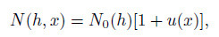
where h is the height above the ground, x is the ground range from the sounder along the Earth surface, N0(h) is the initial electron density profile, and u (x) characterizes the variation in critical frequency along the path. Here, N0(h) is known, and u (x) is an unknown function. Once u (x) is solved and substituted into the expression (1), the two-dimensional electron density distribution N (h, x) can be obtained.
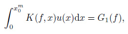
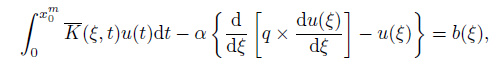
2.3 Inversion ModelWe need to solve the following Fredholm integral equation of the first kind in order to obtain the twodimensional electron density profile described in Section 2.2:
|
(2) |
where K (f, x) is the kernel function, f is the operating frequency, x denotes the x-coordinate (the ground range), x0m is the x-coordinate of the scattering point of a ray with a minimum group path for a spherically stratified ionosphere (hereafter the subscript ‘0' refers to the parameters for a horizontally homogeneous ionosphere), G1(f)= G (f)−G0(f), G (f) is the measured leading edge of a backscatter ionogram, and u (x) is the unknown function.
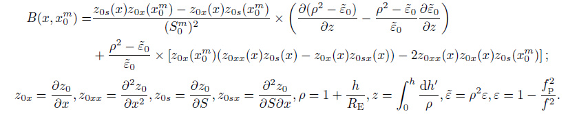
We use the kernel function deduced by Fridman and Fridman (1994) which has the form

|
(3) |
where
|
In the above expressions, fp is the plasma frequency; S = sin β, where β is the ray exit angle, i.e., the angle between the vertical direction and the direction of the propagation; Sm = sin βm, where βm is the ray exit angle of minimum group path (the superscript ‘m' denotes the parameters of minimum group path).
Since the inversion of a backscatter ionogram belongs to the class of ill-posed problems, we have availed ourselves of the Tikhonov regularization method which uses the smoothness condition for the solution as additional information to solve the inverse backscatter sounding problem.
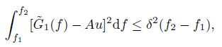
According to the Tikhonov regularization theory, the solution satisfying the following expression (4) is called an approximate solution of the inverse problem (2),
|
(4) |
where
|
(5) |
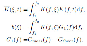
$\tilde{G}$ 1(f) indicates the difference between the experimental leading edge Gmeas (f) and the one constructed theoretically using ray trajectory calculations Gtheor (f), that is, $\tilde{G}$1(f)= Gmeas (f)− Gtheor (f). The variables f1 and f2 are the start and end operating frequencies respectively. The quantity δ is called the residual and is the upper bound of the measurement errors.
The smoothest function $\tilde{u}$ (x) that satisfies the relationship (4) is taken to be the best approximate solution, namely the regularization solution. We use the following form of the functional as the measure of smoothness, which is referred to as stabilizing functional:
|
(6) |
Here, q is a constant, q ≥ 0. And then, the solution $\tilde{u}$ (x) imparting a minimum to the functional (6) when the condition (4) is satisfied, is taken as an optimum solution. It is proved that such optimization problem has a unique solution (Tikhonov et al., 1977). Utilizing Lagrange method of multipliers, the inversion problem is reduced to finding solutions uα minimizing the functional which is called the smoothing Tikhonov functional
|
(7) |
where α is a positive constant called the regularization parameter. The larger the value of α, the greater the weight of the stabilizing functional Ω(u) in the smoothing Tikhonov functional (7) and, consequently, the smoother the solution uα obtained. However, if the value of α is too large, the overly smooth solution will deviate from the true solution. The optimal regularization parameter α is the largest value for which the inequality (4) is satisfied.
2.4 Implementation of the Inversion MethodThis section mainly describes the implementation of the inversion algorithm we proposed. The realization includes the following steps.
(1) Establishment of an ionospheric electron density grid about the region we are interested in. The grid is formed according to the ground range and the height on the backscatter sounding plane, as shown in Fig. 2.

|
Fig. 2 Scheme of an ionospheric electron density grid |
(2) Preparation of input data for the inversion algorithm. The input data include
① Leading edge of a measured backscatter ionogram, Gmeas (f);
② Vertical electron density profile over the backscatter sounding station, N0(h);
③ n a priori values of the leading edge measurement errors. The operating frequency range of the measured backscatter leading edge is divided into n bands, and the length of each frequency band is denoted by Δfi (i = 1, 2, …, n). The a priori values of measurement errors about the leading edge data corresponding to frequency ranges, i.e. [fa, fa +Δf1], [fa, fa + Δf1 + Δf2], …, [fa, fa + Δf1 + Δf2 + … + Δfn] = [fa, fb] are denoted by δ1, δ2, …, δn respectively, generally δ1 ≤ δ2 ≤ … ≤ δn.
The input ② is acquired by the inversion of the vertical sounding ionogram over the backscatter sounding station.
(3) Inversion using the leading edge data Gmeas ([fa, fa + Δf1]) of the frequency range [fa, fa + Δf1]. Since the inversion problem (2) is generally nonlinear, we solve the problem iteratively applying the Newton- Kontorovich method. The specific steps are as follows:
(I) The initial two-dimensional electron density profiles for the grid in Fig. 2 are considered to be horizontally homogeneous, i.e. N (h, x)= N0(h). For this ionosphere, we construct the leading edge Gtheor ([fa, fa + Δf1] for frequency range [fa, fa +Δf1] using the ionospheric numerical ray tracing technique developed by Liu et al. in 2008.
(II) The norm symbol $\left\| {} \right\|$ is used here for root-mean-square value of a function. We define the rms discrepancy between the constructed and measured leading edges as the following expression:
|
(8) |
where M is the total number of the leading edge points in the inversion.
If the condition

|
(9) |
is satisfied, the initial electron density profile specified in step (I) of step (3) gives the optimum solution of the inverse problem. Otherwise, the iterative process described below is started.
(III) We solve the inverse problem (2) corresponding to the leading edge data of frequency range [fa, fa + Δf1].
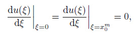
From the Tikhonov regularization method, the inverse problem (2) is equivalent to the problem of finding the solution that minimizes (7), and the solution minimizing (7) may be found by solving the integrodifferential Eq.(10) subject to boundary condition (11) which are expressed as follows:
|
(10) |
|
(11) |
where
|
Here, 
In the above problem, u is the unknown function, K is the known kernel which can be calculated by (3), and the parameter q generally needs to satisfy q ≤ L2, where L is the typical scale of the expected horizontal variation in electron density. Guided by the consideration that the typical scale of a regular horizontal inhomogeneity of the mid-latitude ionosphere is of the order of a thousand kilometers or larger, we put q = 106 km 2 here. It should be noted that, although the selection of parameter q is very important, as long as its value is set within a certain range, the inversion results are not sensitive to it.
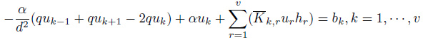
Due to the introduction of the electron density grid, the problem of (10) and (11) can be expressed discretely, and solved numerically from below
|
(12) |
|
(13) |
where
|
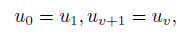
The grid is taken to be uniform. v is the number of mesh points for the ground range grid, w is the number of operating frequencies, d and s are the step of the ground range and the operating frequency, respectively.
At a given α, the solution uαk (k = 1, …, v) corresponding to v unknowns is solved from the above v linear algebraic equations using the Cholesky decomposition method, and it is the discrete form of uα(x). We choose the largest value of α that satisfies (4) as the optimal regularization parameter αd, and its corresponding solution is called the regularization solution, which is the one we desire. Substituting uαd (x) into (1) we obtain the electron density distribution N (h, x) along the path of sounding.
(IV) For the new form of the electron density distribution N (h, x), the theoretical leading edge Gtheor ([fa, fa+Δf1]) of the frequency range [fa, fa+Δf1] is calculated through the ray tracing technique. If Gtheor ([fa, fa+Δf1]) satisfies the condition (9), N (h, x) is the optimum solution of the inverse problem, denoted as N1(h, x)(the superscript ‘1' represents the 1st frequency range, and the same below), and the inversion process of this frequency range is ended. Otherwise, the process returns to step (III) above.
(4) Inversion using the leading edge data Gmeas ([fa, fa+Δf1+Δf2]) of the frequency range [fa, fa+Δf1+ Δf2]. The inversion process is the same as step (3), but need to take N1(h, x) as the initial profile involved in step (I) of step (3) which is the electron density distribution obtained from the leading edge data of the last frequency range. Denote the inversion result of the present frequency range as N2(h, x).
(5) The frequency range is added gradually by way of the division in step ③ of step (2), and then the inversion is implemented using the method described in step (4). After inversion processes (corresponding to n frequency ranges), the final two-dimensional electron density distribution Nn (h, x) is obtained, which is the optimal inversion result of our algorithm. Now, all the inversion work about the algorithm presented in this paper is completed.
3 RESULTS AND ANALYSIS OF THE INVERSION METHOD 3.1 Inversion of Simulated DataThe goal of the present section is to investigate the capabilities of our developed method of diagnosing the inhomogeneous ionospheric structure via simulated data. The testing procedure includes the following stages.
(1) Assuming an ionosphere model with a certain level of inhomogeneous distribution (here considering the disturbed ionosphere model established by Liu et al.(2005)), and regarding the ionosphere model as the "true" ionosphere. Constructing the "measured" backscatter leading edge based on the "true" ionosphere.
(2) Reconstructing the horizontally-inhomogeneous ionospheric structure using the "measured" backscatter leading edge.
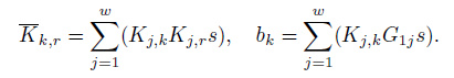
(3) Comparing the reconstructed electron density distribution with the "true" ionosphere. The disturbed ionosphere model by Liu et al.(2005) is written as
|
where NE, NJ, NF are the electron densities of E layer, joining layer and F layer at a distance r from the center of the earth respectively; rEm and rFm are the radial distances where the maximum electron densities of E layer and F layer occur, and rJ = rEm; aE, bE, aJ, bJ, aF, bF are the values of quantities a and b of E layer, joining layer and F layer, a = fc2 /80.6, b = a (rb/ym)2, ym = rm − rb, fc is the critical frequency, rb is the base height of the layer, and ym is the layer semi-thickness.
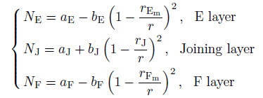
The variation of the critical frequency of F layer with the geocentric angle θ in the above model is described by the following expression
|
(15) |
where v1, v2, v3 are the geocentric angles from the front edge, center and back edge of the ionospheric disturbance to the backscatter sounding station respectively, v = v2 − v1 = v3 − v2, fc (0) is the critical frequency over the sounding station, and characterizes the fluctuation level of the critical frequency in the disturbance zone (MHz/rad).
For the simulation test in this paper, the model parameters are set as follows: fEc = 2.5 MHz, rEb = 6451 km, yEm = 10 km, fFc = 12.4 MHz, rFb = 6571 km, yFm = 130 km, and the disturbance parameters are given by v1=0.035 rad, v2=0.065 rad, v3=0.095 rad, wE=0.1 MHz/rad, wF=0.3 MHz/rad.
We reconstruct the electron density distribution using the method we have developed and the one proposed by Fridman and Fridman (1994). The results are shown in Fig. 3. Fig. 3a presents the "true" distribution of critical frequency of F2 layer (foF2) along the backscatter sounding direction over the distance range of 0~2000 km and that of the reconstructed ones. Fig. 3b illustrates the comparison between the "measured" backscatter leading edge and the theoretically calculated ones.

|
Fig. 3 Comparison between the inversion results of our algorithm and those of the algorithm presented by Fridman and Fridman in 1994 using simulated data (a) Comparison of foF2 inversion results of ground distance 0~2000 km;(b) Comparison of the backscatter leading edges constructed using the inversion results. |
In this example, in order to obtain the "measured" backscatter leading edge, we use the ray tracing technique to construct the leading edge, and superimpose the random noise on it with dispersion σd=20 km which simulates measurement errors. The operating frequency range used here is 5~28 MHz, and is divided into 4 bands. The corresponding parameters are set by Δfi= 5 MHz (i = 1, 2, 3), Δf4=8 MHz, and δi=20 km (i = 1, 2, 3, 4). The size of the electron density grid is 40 × 400, that is, 40 meshes of ground ranges covering 0~2000 km at steps of 50 km, and 400 meshes of heights covering 0~400 km at steps of 1 km. As can be seen from Fig. 3a, there is a significant disturbance in the ionosphere at a distance of about 400 km from the sounding station. The length of the disturbance zone is about 350 km, and the value of foF2 is decreased by 1.9 MHz at the maximum disturbance site. The inversion results by the algorithm of Fridman and Fridman (1994) nicely capture the location of the disturbance zone, but the reconstructed electron density is not accurate enough, where the value of foF2 at the maximum disturbance site is lower than the "measured" value by 0.65 MHz, and at the distances behind the back edge of the disturbance, the values of foF2 also have large errors compared with the "measured" ones. By contrast with the algorithm of Fridman and Fridman (1994), we have obtained better inversion results which show that the discrepancy between the reconstructed foF2 and the "measured" one at the maximum disturbance site is only 0.2 MHz, the positioning of the back edge of the disturbance is more accurate, and the reconstructed electron density distribution at most ground ranges agrees well with the "true" ionosphere. After calculation, we get that the rms errors of the reconstructed values of foF2 over the ground ranges of 0-2000km for our algorithm and the algorithm of Fridman and Fridman (1994) are 0.11 MHz and 0.26 MHz respectively, which demonstrate the overall accuracy of the inversion of the former algorithm is higher than that of the latter one. Fig. 3b indicates that our algorithm constructs a more accurate backscatter leading edge than that of the algorithm of Fridman and Fridman (1994) compared with the "measured" one, particularly in the fluctuating region (12~18 MHz).
3.2 Inversion of Experimental DataTo validate the algorithm presented in this paper for the inversion of experimental backscatter ionograms, we carry out the test using substantial sounding data by the China Research Institute of RadioWave Propagation (CRIRP). Test results demonstrate that our algorithm is effective for the inversion of experimental data, behaves robust, and has strong practicability.
The whole experimental systems are comprised of a backscatter sounder, two vertical sounders (one is for quasi-vertical sounding and referred to as No.1 vertical sounder, and the other is referred to as No.2 vertical sounder) and an oblique sounder. The transmitting equipments of the backscatter sounder and the No.1 vertical sounder are located at A point, and the receiving equipments of the two are located at B point about 100 km apart from A point. The backscatter ionograms and the vertical ionograms at B point can be formed through receiving their respective transmitting signals. The No.2 vertical sounder is set at C point 1000 km apart from B point in the backscatter sounding direction and the vertical ionograms at C point can be obtained. The receiving equipment of the oblique sounder is also situated at B point, and via sharing the transmitting equipment with the No.2 vertical sounder, the oblique ionograms for CB link can be acquired. The schematic diagram of the test system is shown in Fig. 4. The system provides nearly simultaneous measurements of the backscatter ionograms, vertical ionograms and oblique ionograms. The backscatter leading edge and the electron density profiles over the two vertical sounders are calculated using the intelligent interpretation technique for backscatter ionograms (Qi et al., 2011 ; Feng et al., 2012 ; Feng et al., 2014) and the vertical ionogram inversion method (Wei et al., 2015) developed by CRIRP. The backscatter leading edge and the electron density profile over the No.1 vertical sounder are used as input to the inversion algorithm and the two-dimensional electron density distribution over the ground ranges of 0~2000 km in the sounding direction is recovered. The electron density profile over the No.2 vertical sounder is utilized to testify the accuracy of the inversion results over the corresponding ground range site. For the reconstructed two-dimensional electron density profiles, we calculate the oblique ionogram with the ground range of 1000 km by the ray tracing technique and compare with the measured oblique ionogram, in order to test the inversion accuracy of the electron density in the reflection region of the oblique sounding link.

|
Fig. 4 Sketch map of experiment |
Here are two examples for inversion of experimental ionograms. One is for sunset time and the other is for day time.
Figure 5 presents a group of ionograms for synchronously sounding at sunset time, where the leading edge of the backscatter ionogram is marked by a black solid line. During sunrise and sunset periods, the ionosphere tilts which means that the contour lines of the electron density are no longer plane or spherical, and there is a large undulation for the electron density distribution. In Fig. 5, the values of foF2 are 10.8 MHz for the No.1 vertical sounder, and 18.2 MHz for the No.2. The discrepancy of 7.4 MHz between the two sounders indicates that there exist large horizontal gradients within the ionosphere in this direction. This can be also represented by the shape of the leading edge of the backscatter ionogram. It can be seen from Fig. 5a that the backscatter leading edge line is straight, and this corresponds to the ionosphere having positive electron density horizontal gradients in the sounding direction (Jiao, 1990).

|
Fig. 5 Ionograms for backscatter sounding (a), vertical sounding (b) and (d), oblique sounding (c) at 17:25 on 14 December 2014 |
We regard the electron density profile over the No.2 vertical sounder calculated using the vertical ionogram inversion technique suggested by Wei et al.(2015) as the true ionosphere and employ it to test our inversion results at the ground range of 1000 km. As shown in Fig. 6a, the blue asterisked line represents the true electron density profile over the No.2 vertical sounder with the critical frequency of 18.2 MHz, while the red dotted line and the green circled line represent the profiles reconstructed by our algorithm and the algorithm of Fridman and Fridman (1994) with the critical frequencies of 17.8 MHz and 19.6 MHz, respectively. It is apparent that either the critical frequency or the entire profile of the former is closer to the true value than that of the latter. However, we also note that the peak heights (heights of the maximum electron densities) reconstructed by the two algorithms are both slightly lower than the true one with the difference of about 20 km. This is because the peak height of the ionospheric model used in the inversion algorithms (see Section 2.1) is constant (equal to the peak height over the No.1 vertical sounder), whereas the peak height of the true ionosphere usually varies with the ground range. This is one of the contents to further improve our inversion method.

|
Fig. 6 Comparison between the inversion results of our algorithm and those of the algorithm presented by Fridman and Fridman (1994) using measured data at sunset (a) Comparison of electron density profiles over the No.2 vertical sounder;(b) Comparison of the constructed oblique ionograms. |
Figure 6b shows the oblique tracings constructed based on the inversion results by our algorithm and the algorithm of Fridman and Fridman (1994) superimposed on the measured oblique ionogram of Fig. 5c. The maximum usable frequency (MUF) of F2 layer in the measured oblique ionogram is 24.5 MHz, and the MUFs in the oblique ionogram constructed by the two inversion algorithms are 24.2 MHz (our algorithm) and 27.5 MHz (algorithm of Fridman and Fridman (1994)) respectively. It is clear that the MUF constructed by us is very close to the measured value, and the accuracy is improved by 11 percent compared with the algorithm by Fridman and Fridman (1994). As can be seen from the figure, the overall oblique tracing of F2 layer constructed by our algorithm is in reasonable agreement with the measured tracing, except the slightly lower group path which is also due to the use of the ionospheric model with the fixed peak height. However, the constructed oblique tracing of E layer is not consistent with the measured tracing. This is because only the leading edge of F layer is used in both inversion algorithms and the leading edge of E layer is ignored, thus resulting in the reconstructed ionospheric structures containing more information of F layer, less E layer. One solving method is to utilize the backscatter leading edges of E layer and F layer for joint inversion which requires the research on the right joint inversion technique and the development of the effective method for extracting the leading edge of E layer. One of the difficulties is that the leading edge of E layer is generally not well-defined in a measured backscatter ionogram (e.g. Fig. 5a, only the leading edge of F layer can be identified), and this may be achieved by using the model calculation whose feasibility needs to be tested in the follow-up study.
Figure 7 shows the two-dimensional electron density profile inverted over the sounding path. It can be seen that, in the 0~300 km ground distance range, the ionosphere is basically uniform, and with the increasing ground distance, the electron density increases rapidly until at a distance of about 800 km. Then the ionosphere is beginning to take on a steady state.

|
Fig. 7 Two-dimensional electron density profile (during sunset) |
Figure 8 shows a group of ionograms synchronously sounded in the daytime. It is found that at mid-latitudes, the conditions of the ionosphere in the daytime or at night are usually quieter than those during the sunrise or sunset periods. From Fig. 8 we can also see that the difference between the critical frequency of the No.1 vertical sounder and that of the No.2 vertical sounder is only 0.1 MHz, and the minimum virtual heights of each layer over the two sounders are almost the same. These indicate that there exists very small inhomogeneity in the electron densities along the backscatter sounding path, and the ionosphere is approximately spherically stratified. The backscatter leading edge line in Fig. 8a takes on a quadratic curve, and according to Jiao (1990), a quadratic curve of backscatter leading edge commonly corresponds to a spherically stratified ionosphere or an ionosphere with negative horizontal gradients along the path under investigation.

|
Fig. 8 Same as in Fig. 5 but at 9:46 on 10 February 2015 |
Figure 9 shows the same inversion results as in Fig. 6 but in the daytime. As can be seen from Fig. 9a, the electron density profile reconstructed by our algorithm substantially coincides with the true profile except for the peak height of F2 lower by 5 km, while the profile reconstructed by the algorithm proposed by Fridman and Fridman (1994) has a certain deviation from the true one. The electron density profiles of E layer reconstructed by both algorithms are a little inaccurate, and the reason is the same as the discussed above, that is, the backscatter leading edge of E layer doesn't participate in the inversion process. In Fig. 9b, the MUFs of the measured oblique ionogram and the ionograms constructed using algorithms presented in this paper and Fridman and Fridman (1994) are 18.1 MHz, 18.2 MHz and 18.7 MHz respectively. The results indicate that for the ionosphere with a small horizontal gradient of electron density, better inversion results still can be got using the algorithm suggested in this paper than using the method suggested by Fridman and Fridman (1994). It should be noted that when reconstructing the homogeneous ionosphere, we still use the two-dimensional ionospheric model in Section 2.2 which can describe the inhomogeneous electron density distribution, but impose smoothness limitations and constraints on the model space via the algorithm presented in this paper characterized by gradually approaching the solution with increased frequency range and the Eq.(7).

|
Fig. 9 Same as in Fig. 6 but in the daytime |
Figure 10 shows the two-dimensional electron density profile over the daytime sounding path. With the increase of the ground distance, the change of electron density is not obvious, which means that the ionosphere has a very small horizontal electron density gradient.

|
Fig. 10 Two-dimensional electron density profile (in the daytime) |
Fifty ionospheric sounding cases during the period from June 2014 to June 2015 are used in the testing procedure. These cases covering four seasons and four time periods of the sunrise, sunset, daytime and nighttime can fully reflect the diversity of the state of the ionosphere. Comparing the electron density profiles reconstructed by our algorithm and the algorithm of Fridman and Fridman (1994) with the vertical sounding profile measured at the No.2 vertical sounder, we obtain the error statistics of the two inversion algorithms as shown in Fig. 11. We specify the allowable error range of the critical frequency as 0.0~1.0 MHz. The error of more than 1.0 MHz indicates the inversion result is not correct, and the error between 0.0 MHz and 0.5 MHz illustrates that the inversion result is quite accurate. Fig. 11 shows that 86% of the inversion results obtained using our algorithm are within the allowable error range, and the proportion is higher than that of the results obtained by the algorithm suggested by Fridman and Fridman (1994) (80%). Moreover, 70% of the inversion results from the former algorithm are quite accurate, while only 55% for the latter algorithm. It is clear that our algorithm is superior to the algorithm presented by Fridman and Fridman (1994). This inversion test for experimental data demonstrates that either for the quiet ionosphere such as in the daytime or at nighttime, or for the ionospheric horizontally inhomogeneous structures with large horizontal gradients, the algorithm developed in this paper has obtained satisfactory results and is proved to be effective in dealing with the complicated backscatter data sounded experimentally.

|
Fig. 11 Statistics of the inversion results |
In this paper we have used a simplified ionospheric model with an unchanged vertical profile shape. It will be assumed that the shape of the electron density profile remains approximately unchanged along the path under investigation, and only the maximum value of density changes according to the formula (1). This model can be used to describe abrupt, irregular or non-monotonic horizontal changes in electron density observed, for example, in the region of the mid-latitude ionospheric trough, or during both the evening and morning hours on mid-latitude paths. Using the model can impose restrictions on the solution space and reduce the non-uniqueness of the solution, which is beneficial to the stability of the inversion results. The inversion results of the measured backscatter ionograms in this paper are in good agreement with true values, which indicates that the model is reasonable and feasible in practical application.
The inversion technique using backscatter leading edges, which can provide height profile parameters at distances of 1000 km or more from the sounding station, is very effective for determining the spatial variation of medium- and large-scale structures in the ionosphere, and this is crucial for HF radio wave propagation. However, it is noteworthy that not all the ionospheric structures are recovered. In the height range above the maximum reflection height, some disagreement between the true and recovered N (h)-profiles is observed, and this can be illustrated from Fig. 1 which shows that the rays forming the leading edge don't pass through the height range mentioned above and consequently don't contain the corresponding information of electron density. Nevertheless, the height range of the inversion is always sufficient for the needs of supporting the short-wave application systems (such as OTHR, HF communication, etc.). In addition, the error of reconstructing the lower layer of ionization with the heights from 100 km to 200 km is high since only the leading edge of F layer is used in the inversion process. In order to improve the inversion accuracy for the region below F2 layer, it may be necessary to implement the inversion utilizing the leading edges associated with the E and F layers jointly.
5 CONCLUSIONSWe have developed in this paper a method for inversion of backscatter ionograms. Based on the idea of imposing constraints on the solution space, we present the algorithm characterized by gradually approaching the solution with increased frequency range, where an ionospheric model that has the unaltered vertical profile shape everywhere is used and meanwhile the Newton-Kontorovich method for solving nonlinear problems and the Tikhonov regularization method for linear ill-posed problems are applied. The algorithm developed here has higher inversion accuracy and can diagnose the horizontally inhomogeneous structures of the ionosphere effectively. Input data for the inversion procedure include: ① the leading edge of a measured backscatter ionogram; ② the vertical electron density profile measured over the backscatter sounding station; ③ n a priori values of the leading edge measurement errors corresponding to n frequency ranges acquired from the whole operating frequencies, namely, δ1, δ2, …, δn. The output is a two-dimensional distribution of electron density in a vertical plane aligned with the direction of backscatter sounding. In fact, the input of ② can be substituted with the vertical electron density profile measured over some other site lying in the sounding direction.
The method developed in this paper has been tested against both simulated data and experimental data. Fridman and Fridman (1994) proposed a technique of backscatter sounding inversion useful for reconstructing the two-dimensional electron density distribution in the sounding direction. In order to examine the accuracy of our algorithm, we compare our inversion results with those of the algorithm of Fridman and Fridman (1994). The comparison shows that both for the simulated data with severe ionospheric disturbances and for the experimental data with a large gradient in the horizontal direction or approximately horizontally homogeneous, our developed method has a higher inversion accuracy, which demonstrates that our inversion theory is correct and is an effective improvement of the algorithm developed by Fridman and Fridman (1994). Several inversion tests have proven that the algorithm established in this paper can accurately diagnose the horizontally inhomogeneous structure of the ionosphere in the sounding direction and has the ability against data errors, that is, not sensitive to measurement errors of the backscatter leading edge. These merits ensure the application value of the proposed algorithm in the treatment of the complex and volatile measured backscatter ionograms.
ACKNOWLEDGMENTSThis work was supported by the Basic Research Project of National Defense Technology (JSHS2014210A002), the National Natural Science Foundation of China (61331012), and the Technology Innovation Fund Project of CETC (JJ-QN-2013-28).
| [] | Benito E, Bourdillon A, Saillant S, et al. 2008a. Inversion of HF backscatter ionograms using elevation scans. Journal of Atmospheric and Solar-Terrestrial Physics , 70 (15) : 1935-1948. DOI:10.1016/j.jastp.2008.09.031 |
| [] | Benito E, Saillant S, Molini J P, et al. 2008b. Inversion of backscatter ionograms optimization by using simulated annealing and genetic algorithms.//2008 IEEE International Geoscience and Remote Sensing Symposium. Boston, MA:IEEE, Ⅲ-1127-Ⅲ-1130. |
| [] | Caratori J, Goutelard C. 1997. Derivation of horizontal ionospheric gradients from variable azimuth and elevation backscatter ionograms. Radio Science , 32 (1) : 181-190. DOI:10.1029/96RS02026 |
| [] | Chuang S L, Yeh K C. 1977. A method for inverting oblique sounding data in the ionosphere. Radio Science , 12 (1) : 135-140. DOI:10.1029/RS012i001p00135 |
| [] | Coleman C J. 1998. A ray tracing formulation and its application to some problems in over-the-horizon radar. Radio Science , 33 (4) : 1187-1197. DOI:10.1029/98RS01523 |
| [] | Croft T A. 1972. Sky-wave backscatter:A means for observing our environment at great distances. Reviews of Geophysics , 10 (1) : 73-155. DOI:10.1029/RG010i001p00073 |
| [] | DuBroff R E, Rao N N, Yeh K C. 1979. Backscatter inversion in spherically asymmetric ionosphere. Radio Science , 14 (5) : 837-841. DOI:10.1029/RS014i005p00837 |
| [] | Dyson P L. 1991. A simple method of backscatter ionogram analysis. Journal of Atmospheric and Terrestrial Physics , 53 (1-2) : 75-88. DOI:10.1016/0021-9169(91)90022-Y |
| [] | Feng J, Li X, Qi D Y. 2012. Methods for extracting backscatter ionogram leading edges. Chinese Journal of Space Science(in Chinese) , 32 (4) : 524-531. |
| [] | Feng J, Qi D Y, Li X, et al. 2014. Methods for auto-identification of propagation modes from backscatter ionograms. Chinese Journal of Radio Science (in Chinese) , 29 (1) : 188-194. |
| [] | Fridman O V, Fridman S V. 1994a. A method of determining horizontal structure of the ionosphere from backscatter ionograms. Journal of Atmospheric and Terrestrial Physics , 56 (1) : 115-131. DOI:10.1016/0021-9169(94)90181-3 |
| [] | Fridman O V, Nosov V E, Boitman O N. 1994b. Reconstruction of horizontally-inhomogeneous ionospheric structure from oblique-incidence backscatter experiments. Journal of Atmospheric and Terrestrial Physics , 56 (3) : 369-376. DOI:10.1016/0021-9169(94)90218-6 |
| [] | Fridman S V. 1998a. Reconstruction of a three-dimensional ionosphere from backscatter and vertical ionograms measured by over-the-horizon radar. Radio Science , 33 (4) : 1159-1171. DOI:10.1029/98RS00477 |
| [] | Fridman S V, Berkey F T. 1998b. Utilization of sky-wave backscatter sounders for real-time monitoring of ionospheric structure over extended geographic regions. Geophysical Research Letters , 25 (6) : 885-888. DOI:10.1029/98GL00428 |
| [] | Fridman S V, Nickisch L J. 2001. Generalization of ionospheric tomography on diverse data sources:Reconstruction of the three-dimensional ionosphere from simultaneous vertical ionograms, backscatter ionograms, and total electron content data. Radio Science , 36 (5) : 1129-1139. DOI:10.1029/1999RS002405 |
| [] | Fridman S V, Nickisch L J, Hausman M. 2009. Personal-computer-based system for real-time reconstruction of the threedimensional ionosphere using data from diverse sources. Radio Science , 44 : RS3008. DOI:10.1029/2008RS004040 |
| [] | Fridman S V, Nickisch L J, Hausman M. 2012. Inversion of backscatter ionograms and TEC data for over-the-horizon radar. Radio Science , 47 : RS0L10. DOI:10.1029/2011RS004932 |
| [] | Jacquet F, Caratoff J, Dorizzi B. 2001. Derivation of the ionospheric structure over extended geographical regions from azimuth and elevation scan backscatter ionograms:A modular neural network approach. Radio Science , 36 (5) : 1043-1052. DOI:10.1029/2000RS002332 |
| [] | Jiao P N. 1990. The effect of the horizontal density gradient on Pmin(f) curve. Chinese Journal of Radio Science (in Chinese) , 5 (1) : 18-22. |
| [] | Landeau T, Gauthier F, Ruelle N. 1997. Further improvements to the inversion of elevation-scan backscatter sounding data. Journal of Atmospheric and Solar-Terrestrial Physics , 59 (1) : 125-138. DOI:10.1016/1364-6826(95)00167-0 |
| [] | Liu W, Jiao P N, Wang J J, et al. 2005. A study of the disturbance in the ionosphere using ray tracing technology. Chinese J. Geophys. (in Chinese) , 48 (3) : 465-470. |
| [] | Liu W, Jiao P N, Wang S K, et al. 2008. Short wave ray tracing in the ionosphere and its application. Chinese Journal of Radio Science (in Chinese) , 23 (1) : 41-48. |
| [] | Norman R J. 2003. Backscatter ionogram inversion. Proceedings of the International Radar Conference. Adelaide, SA, Australia:IEEE : 368-374. |
| [] | Norman R J, Dyson P L. 2006. HF radar backscatter inversion technique. Radio Science , 41 : RS4010. DOI:10.1029/2005RS003355 |
| [] | Qi D Y, Feng J, Li X. 2011. Algorithms for automatic cleaning of backscatter ionograms. Progress in Geophys. (in Chinese) , 26 (6) : 1925-1930. DOI:10.3969/j.issn.1004-2903.2011.06.005 |
| [] | Rao N N. 1974. Inversion of sweep-frequency sky-wave backscatter leading edge for quasiparabolic ionospheric layer parameters. Radio Science , 9 (10) : 845-847. DOI:10.1029/RS009i010p00845 |
| [] | Rao N N. 1975. Analysis of discrete oblique ionogram traces in sweep-frequency sky-wave high resolution backscatter. Radio Science , 10 (2) : 149-153. DOI:10.1029/RS010i002p00149 |
| [] | Song J, Zhao Z Y, Zhou C, et al. 2011. Inversion of HF sweep-frequency backscatter ionograms. Chinese J. Geophys. (in Chinese) , 54 (8) : 1953-1959. DOI:10.3969/j.issn.0001-5733.2011.08.002 |
| [] | Tikhonov A N, Arsenin V Y. 1977. Solutions of Ill-posed Problems[M]. New York: Halsted Press . |
| [] | Wei N, Liu W, Lu Z X, et al. 2016. The electron density profile inversion for incompletely developed case of F1 layer. Chinese J. Geophys. (in Chinese) , 59 (3) : 778-790. DOI:10.6038/cjg20160302 |
| [] | Xie S G. 2001. A study on the ionospheric parameters of backscatter ionograms[Ph. D. thesis] (in Chinese). Wuhan:Wuhan University. |
| [] | Xiong N L, Tang C C, Li X J. 1999. Introduction to Ionospheric Physics (in Chinese)[M]. Wuhan: Wuhan University Press . |
| [] | Zhu P, Zhou C, Zhang Y N, et al. 2015. F region electron density profile inversion from backscatter ionogram based on international reference ionosphere. Journal of Atmospheric and Solar-Terrestrial Physics , 129 : 111-118. DOI:10.1016/j.jastp.2015.05.003 |