 2016, Vol. 59


2 University of Chinese Academy of Sciences, Beijing 100049, China;
3 BGP, CNPC, Zhuozhou Hebei 072751, China;
4 Exchange School of International Education, Hebei University of Technology, Tianjin 300401, China
4D seismic technology (Nur, 1982; Nur et al., 1984; Nur and Wang, 1987; Greaves and Fulp, 1987; Pullin et al., 1987; Stang and Soni, 1987; Jack, 1997; Calvert, 2005; Foster, 2007) is an essential element of reservoir management (Wiggins and Startzman, 1990). As Houck (2010) pointed out, early in the life of a field, our information is limited, our understanding of the reservoir is very uncertain, and the potential for reducing uncertainty using 4D data is high. The number and value of the decisions that might be affected by the data (for example placement of development wells) also tend to be high. Later in a field life, uncertainty is lower, and fewer options are available for field intervention. Even so, 4D can add value by influencing specific high-value decisions, such as infill-well targets.
In describing a detailed methodology for performing VOI analysis on oil and gas asset-management problems, Coopersmith and Cunningham (2002) note that the value of 4D information is a function of 4D repeatability beside other factors. Houck (2010) demonstrated that lack of repeatability increases the uncertainty in the 4D interpretation results (P70). The value of 4D data decreases while repeatability decreases. Therefor to promote the repeatability is the essential task of 4D seismic data acquisition and processing. In the case of common source energy, the seismic data repeatability is relevant to geometry repeatability (Landrφ, 1999; Eiken et al, 2003; Simt et al, 2005), and relevant to other factors such as ambient nose.
Fortunately, much of the nonrepeatability caused by factors other than geometry can be mitigated by appropriate processing (Johnston 2013, P 75; Helgerud et al., 2011a). Helgerud et al.’s study shows that ideally, each processing flow choice we make improves repeatability. At the very least, we should do no harm. However there is pretty much residual nonrepeatability. Johnston (2013) gave reference and experience showing that processing cannot eliminate the nonrepeatability caused by geometry nonrepeatability and still affect the data after whole processing. Therefor improving repeatability is essential task in the course of acquisition.
In the seismic exploration, people have been facing great challenge for achieving high geometry repeatability, the effort has been huge, and the effect has been obvious. Therefor, in time-lapse seismic or 4D seismic acquisition stage, to ensure the repeatability is the time-lapse seismic substantial task. The challenge to marine towed streamers is more direct. The geometry of baseline is irregular due to the main ambient impact factors such as ocean currents and their change, obstacles and acquisition operations corresponding to them i.e. bin coverage matching between sail lines, while the geometry of monitor survey should repeat the baseline geometry under the circumstance of different and random ocean current. For the repeatability challenge to towed streamers, there were some solution developed (Widmaier et al., 2003, 2005). Eiken et al. (2003) demonstrated that using the same line orientation and direction, steerable-source technology, overlapping streamers, steerable streamers have become conventional solution. Some operators also use cable steering to fan out the far offset slightly, which has the same effect as overlapping the streamers. In areas of extreme variations in feathering, such as the Gulf of Mexico (Ebaid et al. 2008; Ridsdill-Smith et al., 2008), dual-vessel configuration can provide repeatable coverage options by decoupling the sources and receivers. For marine time-lapse seismic survey, alternative acquisition methods were adopted to improve repeatability substantially. There are several published examples (Gouveia et al., 2004; Brechet et al. 2011) in which OBS are used in monitor-survey acquisition and then matched to the baseline survey’s streamer provided under facilities. However OBS is also used in the baseline (Helgerud et al., 2011b)–even if just as a small patch under the facilities. All those stories manifested the effort for and method of the geometry repeatability and reflected the importance of implementation of geometry repeatability. Naturally the analysis and evaluation is also of importance.
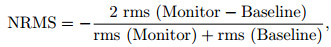
1.1 Seismic Data RepeatabilityMeasures of image repeatability are evaluated over a time window of the data and away from producing zone. The most commonly quoted measure of repeatability in the literature is the normalized RMS difference (NRMS)(Kragh and Christie, 2002; Cantillo, 2011). The NRMS value is simply the RMS amplitude of the difference, normalized by the average of the RMS amplitudes of the baseline data Baseline and monitor data Monitor:
|
(1) |
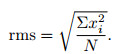
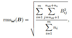
where the rms operator is defined as
|
(2) |
The summation is over N number of all samples xi(i=1, 2, …, N) in the time window.
The NRMS value is a measure of nonrepeatability. If NRMS=0, the data are perfectly repeatable. If the traces from the baseline and monitor seismic are anticorrelated, NRMS=2. Typical “good” values of NRMS quoted in the literature range from 0.1 to 0.3 (10% to 30% nonrepeatability) (Johnston, 2013).
1.2 Geometry RepeatabilityLandrφ, 1999 use data from a VSP experiment to explore further the influence of geometry on repeatability. The NRMS of two traces recorded at the same receiver from two shots separated by less than 5 m is 8%. Landrφ, 1999 studied the spatial correlation in nonrepeatability using NRMS values from 87125 shot pairs. There is certainly a trend of increasing nonrepeatability as the shot separation increases.
Differences in source and receiver positions result in different repeatabilities because of different raypaths through the overburden and different illumination of the target. Eiken (2003) took a seismic survey, shifted it laterally one bin (25 m), and then substracted it from the original survey. The differences are significantly 40% NRMS. The heterogeneity in the overburden affects the repeatability sensitivity to difference of geometry. Smit et al. (2005) plot NRMS values as a function of ∆S + ∆R for 4D surveys. In any event, there is a clear trend of decreasing NRMS values (increasing repeatability) with decreasing values of ∆S + ∆R. Difference in source and receiver positions (∆S + ∆R) is the most commonly quoted measure geometry repeatability. Misaghi et al. (2007) demonstrate that for the same source separation, raypaths that pass through a seismic heterogeneity identified on 3D seismic data have higher NRMS values than raypaths that pass through a more homogeneous overburden, thereby suggesting that increased overburden complexity degrades repeatability. That relationship is likely to be more pronounced in a surface seismic survey than in a VSP because raypaths travel through the overburden twice. Previous studies commonly appeal to cross-equalization processing to mitigate the difference (Li and Hu, 2004; Jin et al., 2005a, 2005b; Jin and Chen, 2003, 2005; Hao and Chen, 2007; Su et al., 2009a, 2009b; 2009c; Hu et al., 2003; Gan et al., 2003; Li et al., 2008), but because of the reason stated by Misaghi, we shall reduce geometry differences to upgrade the consistence or repeatability.
Above-mentioned previous studies show that geometry repeatability namely ∆S + ∆R obviously affect repeatability of time-lapse seismic data, and the effect will be not removable, in other words, geometry repeatability is also a permanent attribute of seismic data.
With the purpose of studying multi-trace situation, and considering the uncertainty of match between monitor and baseline data and different number of traces, Dong (personal communication, 2015; 20151), 2016) came up with the weighted RMS repeatability of the best baseline-based match with imaginary data for mismatch and the weighted RMS geometry repeatability of the best baseline-based match with extrapolation for mismatch.
1) DONG F S. 2015. Research on Survey Repeatability in Time-lapse Seismic. // Report within BGP, CNPC. Tianjin: BGP CNPC.
2 MATCHED MULTI-TRACE GEOMETRY REPEATABILITYIn the time-lapse seismic data acquisition, the geometry repeatability is directly observed, so it is necessary to control the geometry repeatability. Landrφ’s calculation is clear for single pair of traces (1999). Eiken (2003) calculated the repeatability for two seismic sections with clear match of equivalent traces according to CMP using formula (1) and (2). In the acquisition process and before processing, the seismic data is unstacked, so matching of traces corresponding to the same CMP is also generally not completely determined. For the geometry, in the process of monitor data acquisition process, the geometry of pre-stack seismic data is directly observed.
As shown in Fig. 1a, shot point deviation and its inline and cross-line components are much smaller than the inline and cross-line shot intervals, so the match between the monitor and baseline of the shot points is clear. Therefore shot point deviation and its inline and cross-line components can be simply displayed uniquely corresponding to shot points as examples demonstrated by Dong et al. (2013). Based on unique matching of shot points of baseline and monitor, deviations of feather angles can be calculated to measure the deviation of multiple receivers. Hence, geometry repeatability or deviation distribution of monitor survey can formally be profiled and monitored on two planes. However, in fact, there is a certain approximation of itself. As the statistical results shown in Fig. 1b, the vast majority of the receiver point deviations are greater than bin width or half the streamer separation, even a considerable part of the receiver points deviate over the streamer separation. This leads to some shot-receiver midpoints deviating from the bins of midpoints of nominally corresponding baseline shots and receivers into other bins. The receiver points also are far away from the corresponding baseline receiver points and closer to the other points of corresponding shots, as shown in Fig. 1c. This needs to re-match Baseline and Monitor according to the actual spatial relationship or repeatability, and then calculate the repeatability based on the matching relationship. So it is necessary to match and to characterize geometry repeatability based on bins. As in literature (Johnston, 2013), for a chosen single offset, the distribution plane of geometry repeatability can be obtained as a color slice in the cube in Fig. 2. However, to obtain the repeatability of all offset, a three-dimensional data body will be formed. As the quality of time-lapse seismic data, especially for the repeatability monitoring, the geometry repeatability of all offsets or of certain offset range expressed as a distribution on a single acquisition surface is very useful (Fig. 2). This calls for characterization methods and its basis of multi-trace geometry repeatability.

|
Fig. 1 Position deviation (a) Shot point deviation, ∆S: radial deviation, ∆Sx: cross-line deviation, ∆Sy: inline deviation; (b) Receiver point deviation, ∆R1: near trace deviation, ∆R2: near-mid trace deviation, ∆R3: mid-far trace deviation, ∆R4: far trace deviation; (c) Receiver deviation causes middle point’s moving to adjacent bin. |

|
Fig. 2 Acquisition surface-offset space The color slices in the 3D space are displays of geometry repeatability over the acquisition surface for given single offsets. The green 2D plane is a expected display of repeatability for full offset. |
We have statistics on monitor geometry data against baseline data. The monitor acquisition is configured as Table 1.
|
|
Table 1 Configuration of the acquisition for the studied data |
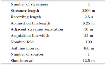
Table 1 shows the configuration of the offshore streamer time-lapse seismic survey from which the actual data used in this paper is derived, and for other relevant background and practice research, see the literature of Dong et al. (2013).
3 THE BASIC THEORYThe theoretic basis of this paper, the weighted RMS repeatability of the best baseline-based match with imaginary data for mismatch and the weighted RMS geometry repeatability of the best baseline-based match with extrapolation for mismatch (Dong, 2015. Personal communication; Dong, 2015, 2016), is described as follows.
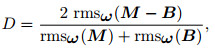
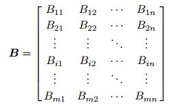
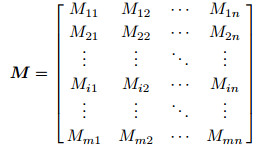
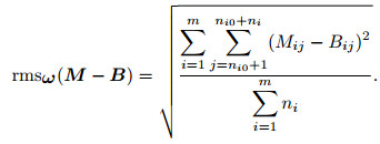
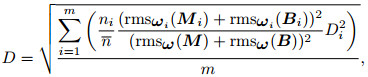
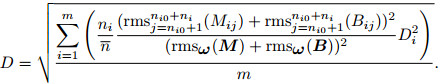
Using structured data B to represent the baseline seismic data, M to represent the monitor seismic data, and D to represent NRMS, formulas (1) and (2) are extended to followings for multi-trace data.
|
(3) |
where
|
(4) |
and
|
(5) |
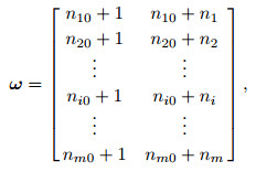
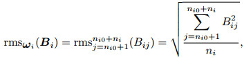
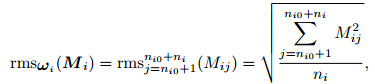
presents baseline and monitor seismic data respectively, whose rows are traces, and ω represent the scope of RMS calculation, or so called space-variant time windows and can be expressed as
|
(6) |
whose value of first and last column in each row indicate the begin and end column number of the window respectively for the same rows in B and M. So
|
(7) |
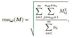
|
(8) |
|
(9) |
Make symbolization as
|
(10) |
|
(11) |
|
(12) |
and correspondingly
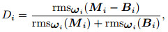
|
(13) |
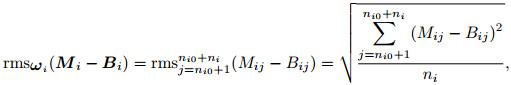
which is repeatability of single pair of traces of rows i in M and B. Then
|
(14) |
Let
|
(15) |
so
|
(16) |
or
|
(17) |
Let

|
(18) |
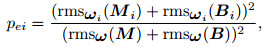
|
(19) |
and

|
(20) |
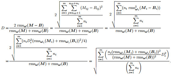
then yield
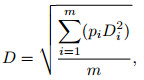
|
(21) |
which indicates that multi-trace repeatability in given windows is the weighted RMS of repeatability of each single pair of traces.
A full permutation
|
(22) |
from 1, 2, …, m without duplicate elements (Yang, 2012) constructs a single column matrix
|
(23) |
referred to as matching vector, where fi≠fk(i≠k), and every element is selected from 1, 2, …, m.
Set m row baseline data matrix B, m' row monitor data matrix M. Define a new m row matrix M(B, M, f), where its row i is row fi of M, and here it is referred to as matched data based on B, where row i of M(B, M, f) or Mi(B, M, f) represents a matched single trace of row i of B or Bi. The situation of absence of row fi in M is referred to as mismatch and row i of M(B, M, f) is an imaged new row uncorrelated with Bi and has the same RMS as Bi. The method of the data supplement is referred to as imagination for mismatch and construction of M(B, M, f) is referred to as baseline-based matching with imaginary data for mismatch. To sum up, the imaginary Mi(B, M, f) meets the condition

|
(24) |
where Mi(B, M, f) presents row i of M(B, M, f).
For baseline-based matched M(B, M, f), there is
|
(25) |
and
|
(26) |
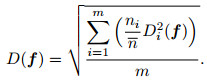
where Di2(f)=(Di(f))2=(D(f))i2. Without new symbols introduced ensuring no confusion to be made, let
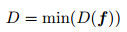
|
(27) |
which is referred to as time-lapse repeatability of the best baseline-based match with imaginary data for mismatch.
When

|
(28) |
there is
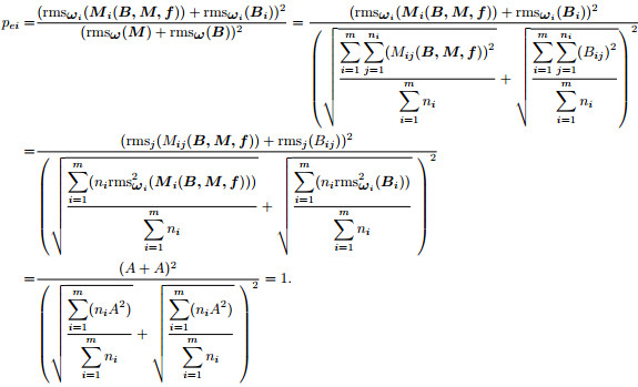
|
(29) |
Therefore
|
(30) |
and then
|
(31) |
Based on previous researches on the relationship of time-lapse seismic data repeatability and geometry repeatability (Landrφ, 1999; Eiken et al., 2003; Smit et al., 2005; Misaghi et al., 2007), utilizing real data from aforementioned survey, repeatabilities of 36 pairs of seismic traces were plotted in Fig. 3a and slope of the fitted line k=0.018/m.

|
Fig. 3 Repeatability of seismic data and its geometry |
Here the real data differs from data from Landrφ, 1999, Smit et al. (2005) and Eiken et al., and k value is bigger for the data comes from shallow water area. This is consistent with the explanation given by Calvert (2005). On the other hand, in the data any shot point deviates in the same direction as the corresponding receiver point (sketched on Fig. 3b), and any CMP deviates in the same extent as the corresponding shot point and receiver point, so this accounts for why k is bigger partly.
The fitted linear relationship within the scope of real data can be formulized as
|
(32) |
where k is a constant relative to the area, di(f) is the geometry repeatability of trace i namely the sum of deviations of the shot point and the receiver point, so
|
(33) |
and let
|
(34) |
then
|
(35) |
Therefor

|
(36) |
Utilizing d again without confusion, define
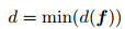
|
(37) |
as the (weighted RMS) geometry repeatability of the best baseline-based match with extrapolation for mismatch. If Mi(B, M, f) is a imaginary row in M(B, M, f), the corresponding geometry match and di(f) does not exist (geometry mismatch). di(f) takes the value d0, which is determined by formula (38) and (39) (so called extrapolation for mismatch). Let D0(√2) represent seismic data repeatability between baseline single trace and monitor imaginary trace, and let d0 be the single trace geometry repeatability of mismatch, then let

|
(38) |
or
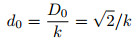
|
(39) |
to determine the value of mismatched single trace geometry repeatability, which is applied to formula (32) to (37), and is referred to as extrapolation for mismatch.
Under the energy balance condition represented by formula (28) and the linear model of the relationship between single trace seismic data and geometry repeatability, supported by definition and relationship, formula (37) gives multi-trace geometry repeatability, which is equivalent to multi-trace seismic data repeatability represented by formula (27) only with a constant coefficient difference.
Actual value range (Landrφ, 1999; Eiken et al., 2003; Smit et al., 2005; Misaghi et al., 2007) of di within which the linear model of the relationship between single trace seismic data and geometry repeatability is formulized by the formula (32) is limited. Whereas, the match trying and selection, and unreasonable data range may result in overlarge d0 value. If consider di bigger than d0 as mismatch, this problem can be avoided and the search range of di < d0 can reduce computing.
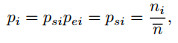
4 VALUE DETERMINATIONS OF pi, k AND d0For multifold seismic data, we can determine the weighting coefficient pi according to valid data after NMO correction and stretch muting.
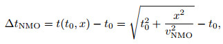
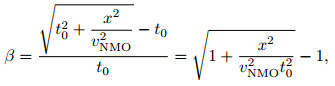
MNO stretch coefficient β (Mu et al., 2007) is determined by
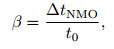
|
(40) |
where ∆tNMO is normal moveout and t0 is two-way zero-offset time.
The reflection traveltime
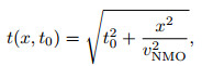
|
(41) |
which is a function of offset x and where vNMO is the velocity of the medium above the reflecting interface.
Thus
|
(42) |
then
|
(43) |
where vNMO=vNMO(t0).
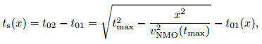
On the basis of time-offset equation (Mu et al., 2007), top muting time t01 ensuring NMO stretch not to exceed given value of β satisfies the equation about x
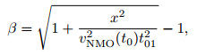
|
(44) |
where vNMO(t0) is NMO velocity, and vNMO2 (t0) represent (vNMO(t0))2. After NMO correction, as a proximate solution, the end time t02 is
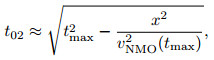
|
(45) |
where tmax is the maximum time in the seismic trace namely the length of seismic trace.
The valid time length is
|
(46) |
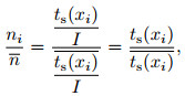
so we obtain
|
(47) |
where I is sampling interval.
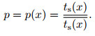
The formula (47) shows that pi varies with offset, so it is represented as
|
(48) |
Via

|
(49) |
and k=0.018/m obtained from the data showed on Fig. 3, d0=80 m can be determined.
5 APPLICATION STUDY ON TOWED STREAMER ACQUISITIONWe employed the velocity function

|
(50) |
and NMO stretch coefficient β=0.2, 0.3, and 0.4, respectively, to calculate the p-offset curves, with the recording length being 2.5 s for the data we used. The curves and p=1 line are showed in Fig. 4.

|
Fig. 4 Weighting coefficient curves |
For the application study, we extracted geometry data from a set of time-lapse project data (nominal shot interval: 12.5 m; nominal offset interval: 25 m), and calculated the multi-trace geometry repeatability according to Eq.(37) and supporting equations, with the matching confined to each single CMP bin. The search intensity in the computing process was reduced based on the condition of the real data. Fig. 5 shows 4 versions of CMP bin repeatability display for the 4 curves of 4 weighting coefficients respectively. In the display, high value means low repeatability, vice versa. The red low repeatability area exhibits the feature of focusing and differentiation when the curve adopted becomes more gradient. It might be due to the repeatability reduced along with offset increased. Once offset-variation weighting coefficient is adopted, the overall repeatability weights near offset much more and the contribution of near and far offset geometry is reasonably and consistently balanced, which reconciles the weak control of long offset geometry repeatability and is supported by relevant theory. The theory will be published in more detail.

|
Fig. 5 Weighted RMS geometry repeatability of the best baseline-based match with extrapolation for mismatch |
For contrast purpose we ignored the mismatched baseline geometry traces and calculated bin repeatability for the same data as in Fig. 5 with p=1 and β=0.2, respectively. The result is displayed in Fig. 6, in which the repeatability in the elliptical circles turns to low value from high value in the corresponding circles in Fig. 5. This is due to mismatched baseline geometry was not taken into account for repeatability while the reserved geometry was well contented with repeatability and gives the false appearance of high repeatability. Therefore this reflects the repeatability computed according to Eq.(37) including extrapolation for mismatch reflects not only geometry repeatability of monitor line but also the coverage repeated for baseline. The significance of repeated coverage is that qualified baseline coverage must meet the designed requirement of coverage even without previous acquisition to be repeated, and the subsequent monitor acquisition’s fold of coverage is the necessary requirement of the 4D acquisition just as single 3D seismic. It is inadequate that only geometry repeatability of monitor amounts to high level, because there is data from baseline that might be not repeated at all. On the contrary, when monitor data has high redundancy and the coverage of baseline is mature, the worst repeating data from monitor is abandoned while the repeatability is computed according to the method argued for in this report.

|
Fig. 6 Weighted RMS geometry repeatability of the best baseline-based match without extrapolation for mismatch |
In Fig. 7, we compared monitor coverage to bin repeatability of baseline-based best match with extrapolation for mismatch for the data or area. It shows that there is extreme low repeatability at the positions corresponding to those where coverage is poor in the coverage map for same area, which proves that bin repeatability of baseline-based best match with extrapolation for mismatch does reflect coverage of monitor survey. In the Fig. 7, we provide normal bin coverage (b) and flexed bin coverage (c) maps. Weighting coefficient selection corresponds to bin flexing, but the response of repeatability to weighting coefficient is weaker than that of coverage to the bin flexing, because bin flexing can eliminate the cavities among bins whereas high value of repeatability cannot vanish by means of lower weighting coefficient for far offset. Generally speaking, the multi-trace geometry repeatability of baseline-based best match with extrapolation for mismatch can reveal the repeatability and fold of coverage simultaneously and can form different repeatability measurement between near and far offset geometry by means of changing weighting coefficient as bin flexing for coverage.

|
Fig. 7 Comparison of geometry weighted RMS repeatability and coverage |
(1) This paper discusses multi-trace seismic data repeatability and its calculation formulae with spacevariant time window, and the theory that multi-trace repeatability is weighted RMS of single trace repeatability. The weighted coefficient is put forward in both expression and calculation. The match for multi-trace repeatability may face the issue of uncertainty and deficiency, so weighted RMS geometry repeatability of baseline-based best match with extrapolation emerged to address the issue properly while the expression can be derived from the NRMS formula. Based on linear model of relationship between seismic data repeatability and geometry repeatability, the weighted RMS geometry repeatability of the best baseline-based match with extrapolation for mismatch was obtained as the equivalent of the repeatability of the best baseline-based match with imaginary data for mismatch.
(2) Regarding application study, the geometry matching was limited to each bin. The study, based on data extracted from real data, and display and parameter contrast, shows that the CMP-bin-based weighted RMS geometry repeatability of baseline-based best match with extrapolation for mismatch can reveal the valid repeatability and coverage of monitor survey simultaneously. So it is a new evaluation technology with new function. It is promising and is expected to be utilized in monitor data acquisition because of concentrated information displayed.
ACKNOWLEDGMENTSIt is in the Institute of Geology and Geophysics (IGG) of Chinese Academy of Sciences and BGP, CNPC where the first author DONG conducted the research and put forward the new theory described in this paper. The research has shared the support from seismological research team of IGG and the technical team of BGP. I send my thanks here. This work is supported by the National Major Science-technology Project (2016ZX05024007).
| [] | Brechet E, Sadeghi E, Giovannini A, et al. 2011. Practice and discussion about towed-streamer 4D seismic data acquisition. Seismic monitoring combining nodes and streamer data on Dalia field.//73rd EAGE Conference and Exhibition, EAGE, Extended Abstracts. SPE, EAGE. |
| [] | Calvert R. 2005. Insights and methods for 4D reservoir monitoring and characterization. SEG Distinguished Instructor Series No.8. SEG. |
| [] | Cantillo J. 2011. A quantitative discussion on time-lapse repeatability and its metrics.//81st Annual International Meeting, SEG, Expanded Abstracts. San Antonio, Texas:SEG, 4160-4164. |
| [] | Coopersmith E M, Cunningham P C. 2002. A practical approach to evaluating the value of information and real option decisions in the upstream petroleum industry.//SPE Annual Technical Conference and Exhibition. San Antonio, Texas:SPE. |
| [] | Dong F S, Quan H Y, Luo M X. 2013. Practice and discussion about towed-streamer 4D seismic data acquisition.//Chinese Geophysics 2013-12th subject. Beijing:Chinese Geophysical Society, 404-407. |
| [] | Dong F S. 2016. Research on survey repeatability in time-lapse seismic[Ph. D. thesis]. Beijing:University of Chinese Academy of Sciences, Institute of Geology and Geophysics, Chinese Academy of Sciences. |
| [] | Ebaid H, Tura A, Nasser M, et al. 2008. First dual-vessel high-repeat GoM 4D survey shows development options at Holstein field. The Leading Edge , 27 (12) : 1622-1625. DOI:10.1190/1.3036965 |
| [] | Eiken O, Haugen G U, Schonewille M, et al. 2003. A proven method for acquiring highly repeatable towed streamer seismic data. Geophysics , 68 (4) : 1303-1309. DOI:10.1190/1.1598123 |
| [] | Foster D G. 2007. The BP 4-D story:Experience over the last 10 years and current trends.//International Petroleum Technology Conference. Dubai, U.A.E.:International Petroleum Technology Conference. |
| [] | Gan L D, Yao F C, Zou C N, et al. 2003. 4-D seismic in water flooding reservoirs:Post-stack cross equalization processing. Progress in Exploration Geophysics , 26 (1) : 54-60. |
| [] | Gouveia W P, Johnston D H, Solberg A. 2004a. Remarks on the estimation of time-lapse elastic properties:The case for the Jotun field, Norway.//74th Annual Internal Meeting, SEG, Expanded Abstracts. Denver, Colorado:SEG, 2212-2215. |
| [] | Gouveia W P, Johnston D H, Solberg A, et al. 2004b. Jotun 4D:Characterization of fluid contact movement from time-lapse seismic and production logging tool data. The Leading Edge , 23 (11) : 1187-1194. DOI:10.1190/1.1825941 |
| [] | Greaves R J, Fulp T J. 1987. Three-dimensional seismic monitoring of an enhanced oil recovery process. Geophysics , 52 (9) : 1175-1187. DOI:10.1190/1.1442381 |
| [] | Hao Z J, Chen X H. 2007. A study on time-lapse seismic cross-equalization QC method based on correlation parameters. Progress in Geophysics (in Chinese) , 22 (3) : 929-933. |
| [] | Helgerud M B, Miller A C, Johnston D H, et al. 2011a. 4D in the deepwater Gulf of Mexico:Hoover, Madison, and Marshall fields. The Leading Edge , 30 (9) : 1008-1018. DOI:10.1190/1.3640524 |
| [] | Helgerud M B, Tiwari U, Woods S, et al. 2011b. Optimizing seismic repeatability at Ringhorne, Ringhorne East, Balder and Forseti with QC driven time-lapse processing.//81st Annual International Meeting, SEG, Expanded Abstracts. San Antonio, Texas:SEG, 4180-4184. |
| [] | Houck R T. 2010. Value of geophysical information for reservoir management.//Methods and Applications in Reservoir Geophysics, Chapter 1:Reservoir Management and Field Life Cycle. SEG Investigations in Geophysics No. 15, 29-36. |
| [] | Hu Y, Liu Y, Gan L D. 2003. 4-D seismic in water flooding reservoirs:Pre-stack cross equalization. Progress in Exploration Geophysics , 26 (1) : 49-53. |
| [] | Jack I. 1997. Time-lapse seismic in reservoir management. SEG Distinguished Instructor Series No. 1. SEG. |
| [] | Jin L, Chen X H. 2003. Effects of time-lapse seismic non-repeatability and verification of cross-equalization processing. Progress in Exploration Geophysics , 26 (1) : 45-48. |
| [] | Jin L, Chen X H. 2005. Processing technique of mix factor in time-lapse seismic cross-equalization method. Oil Geophysical Prospecting , 40 (4) : 400-406. |
| [] | Jin L, Chen X H, Li J Y. 2005a. A new method for time-lapse seismic matching filter based on error criteria and cyclic iteration. Chinese J. Geophys. (in Chinese) , 48 (3) : 698-703. |
| [] | Jin L, Chen X H, Liu Q C. 2005b. New method for time-lapse seismic matching based on SVD. Progress in Geophysics(in Chinese) , 20 (2) : 294-297. |
| [] | Johnston D H. 2013. Practical Applications of Time-lapse Seismic Data. SEG Distinguished Instructor Series No. 16. SEG. |
| [] | Kragh E, Christie P. 2002. Seismic repeatability, normalized rms, and predictability. The Leading Edge , 21 (7) : 640-647. DOI:10.1190/1.1497316 |
| [] | Landr M. 1999. Repeatability issues of 3-D VSP data. Geophysics , 64 (6) : 1673-1679. DOI:10.1190/1.1444671 |
| [] | Li R, Hu T Y. 2004. Cross-equilibration technique in time-lapse seismic data processing. Oil Geophysical Prospecting , 39 (4) : 427. |
| [] | Li Z C, Han L G, Zhang F J, et al. 2008. Cross-equalization technique for time-lapse seismic. Journal of Jilin University(Earth Science Edition) , 38 (S1) : 68-71. |
| [] | Mu Y G, Chen X H, Li G F. 2007. Seismic data processing technique[M]. Beijing: Petroleum Industry Press . |
| [] | Misaghi A, Landr M, Petersen S A. 2007. Overburden complexity and repeatability of seismic data:Impacts of positioning errors at the Oseberg field, North Sea. Geophysical Prospecting , 55 (3) : 365-379. DOI:10.1111/gpr.2007.55.issue-3 |
| [] | Nur A M. 1982. Seismic imaging in enhanced recovery.//SPE Enhanced Oil Recovery Symposium. Tulsa, Oklahoma:SPE, 99-109. |
| [] | Nur A M, Tosaya C, Vo-Thanh D. 1984. Seismic monitoring of thermal enhanced oil recovery processes.//54th Annual International Meeting, SEG, Expanded Abstracts. Atlanta, Georgia:SEG, 337-340. |
| [] | Nur A M, Wang Z. 1987. In-situ seismic monitoring EOR.//SPE Annual Technical Conference and Exhibition. Dallas, Texas:SPE. |
| [] | Pullin N, Matthews L, Hirsche K. 1987. Techniques applied to obtain very high resolution 3-D seismic imaging at an Athabasca tar sands thermal pilot. The Leading Edge , 6 (12) : 1015. |
| [] | Ridsdill-Smith T, Flynn D, Darling S. 2008. Benefits of two-boat 4D acquisition, an Australian case study. The Leading Edge , 27 (7) : 940-944. DOI:10.1190/1.2954036 |
| [] | Smit F, Brain J, Watt K. 2005. Repeatability monitoring during marine 4D streamer acquisition.//67th Conference and Exhibition, EAGE, Extended Abstracts. SPE, EAGE. |
| [] | Stang H R, Soni Y. 1987. Saner Ranch pilot test of fractures assisted steamflood technology. Journal of Petroleum Technology , 39 (6) : 684-696. DOI:10.2118/13036-PA |
| [] | Su Y, Yu S X, Huang Q. 2009a. Cross-equalization technique in 4-D seismic data processing. Xinjiang Geology , 27 (2) : 191-194. |
| [] | Su Y, Li G F, Huang Q. 2009b. Cross-equalization technique and its applications. Xinjiang Petroleum Geology , 30 (5) : 633-636. |
| [] | Su Y, Li L M, Liu Y H, et al. 2009c. Cross-equalization technique and its applications in time-lapse seismic data processing. Geophysical Prospecting for Petroleum , 48 (3) : 247-251. |
| [] | Widmaier M, Hegna S, Smit F, et al. 2003. A strategy for optimal marine 4D acquisition.//73rd Annual International Meeting, SEG, Expanded Abstracts. Dallas, Texas:SEG, 1533-1536. |
| [] | Widmaier M, Long A, Danielsen B, et al. 2005. Recent experience with 4D marine seismic acquisition. First Break , 23 (6) : 77-82. |
| [] | Wiggins M L, Startzman R A. 1990. An approach to reservoir management.//SPE Annual Technical Conference and Exhibition. New Orleans, Louisiana:SPE. |
| [] | Yang Y F, Zhang Z H, Xu Y. 2012. Linear Algebra[M]. Beijing: Science Press . |