 2016, Vol. 59


Turbulence is the main form of movement in surface layer causing exchange and transport of water vapor, CO2 and energy between land surface and atmosphere which have been paid wide attention (Jiang et al., 2013a; Liu et al., 2005a, 2005b; Xu et al., 2008). There have been 683 sites in the global flux observatory network FLUXNET up to April 2014 (http://fluxnet.ornl.gov/). Eddy covariance method (EC) could be widely used for long-term continuous observation of CO2, water vapor, and heat flux exchange between land surface and atmosphere, and has been used by the global FLUXNET network (Baldocchi et al., 2001). EC is built on some basic theoretical assumptions, such as the stationarity of turbulence, homogeneity of underlying, fully developed turbulence and existence of the constant flux layer (Foken and Wichura, 1996), however, these assumptions cannot be met under complicated underlying of Loess Plateau. Rolling terrain has an important effect on the EC measurement (Wang et al., 2007). Much attention has been paid to acquire high quality surface turbulent from Earth scientists (Ding et al., 1997; Liu et al., 2005c, 2009; Jiang et al., 2013b). Many researchers have studied the turbulent data processing and quality control. Mauder et al. (2006) found 80% of the total data are of high quality for latent heat flux from overall quality test of 14 sites measuring data in LITFASS-2003. Göckede et al. (2008) applied a site evaluation approach combining Lagrangian stochastic footprint modeling with a quality assessment approach to 25 forested sites of the CarboEurope-IP network to analyze the spatial representativeness of the flux measurements, instrumental effects on data quality and the performance of the coordinate rotation method. Wang et al. (2009) discussed the impact of different coordinate rotations on friction velocity (u*), sensible heat, latent heat flux, stationarity test and integral turbulent characteristics test (ITC) at oases and desert station, respectively. Zhu et al. (2004) analyzed the error generated by non-vertical installed instrument under non-flat and heterogeneous underlying when using EC, moreover discussed the correction effects and application conditions of different coordinate rotations. On flat and homogeneity surface, Chen et al. (2008) found that the planar fit method (PF) is superior to triple rotation (TR). Jiang et al. (2012) used turbulence, net radiation and soil data from International Energy Balance Experiment (EBEX-2000) to study the characteristics of sensible and latent heat flux under thermal internal boundary layer which is induced by heterogeneous irrigation, at the same time energy balance closure on irrigated days was compared with that on non-irrigated days. Semi-arid areas of Loess Plateau cover a vast area in which the land-atmosphere interaction not only have a non-negligible effect on the formation of arid climate in the northwest of China and the East Asian monsoon circulation, but also play a important role in the change of global climate and atmosphere circulation (Yang and Shao, 2000). Land-atmosphere interaction in this region has become one of the important and urgent fundamental scientific issues to be solved. The rolling terrain, sparse vegetation, and heterogeneous surface of Loess Plateau produce complicated turbulence, while little attention has been paid to the turbulent data processing and quality control. Acquiring high quality surface turbulent fluxes is necessary for providing insight into the characteristics of land-atmosphere interaction in Loess Plateau.
This paper mainly focuses on the effects of various procedures of EC flux corrections on turbulent fluxes in the complicated terrain over Loess Plateau. Data processing and quality control including sonic temperature correction, coordinate rotations, WPL correction (correction for density fluctuations), stationarity test, ITC test, and overall quality classification are used on the 10 Hz raw data from 1 November to 21 November 2008 of Semi-Arid Climate and Environment Observatory of Lanzhou University (SACOL) for effectively improving the quality of turbulent data by reducing additional error due to complicated terrain. We analyze the applicability of double rotation (DR), PF and fetch planar fit (FPF) according to different wind direction, further investigate the characteristics of turbulence in surface layer over complicated terrain such as SACOL.
2 OBSERVATION DATASACOL was established in 2005. It is located at 35.946°N, 104.137°E, and an altitude of 1965.8 m, about 48 km from the center of Lanzhou which is located at the semi-arid region of China. The topography around the site is characterized by the Loess Plateau consisting of plain, ridge and mound, etc., with the elevation ranging between 1714~2089 m. The soil parent material is mainly Quaternary aeolian loess with the main soil type being sierozem. With the international advanced observation instruments, SACOL as one of the reference sites of the international Coordinated Energy and Water Cycle Observations Project (CEOP) is the second long-term observation station over semi-arid areas constructed by China following the Chinese Academy Jilin Tongyu station (Huang et al., 2008; Liang et al., 2014).
The terrain where the measurements are carried out is flat, about 200 m in east-west direction and about 1000 m in north-south direction. Dominant species covering the surface are stipa bungeana as well as artemisia frigida and leymus secalinus. The vegetation height in winter is about 0.10 m (Huang et al., 2008; Liang et al., 2014).
The turbulent flux measurement system consists of a three-axis sonic anemometer (CSAT3, Campbell) measuring u, v, w and sonic temperature Ts and an opened path infrared CO2 and H2O analyzer (LI7500, LICOR) measuring water vapor and CO2 density. These observations are taken at 3.0 m above the ground with signals acquired by a data logger (CR5000, Campbell) at 10 Hz.
Observational instruments are calibrated in the summer of 2008, thus data thereafter are reliable. The 10 Hz raw data during 1-21 November 2008 are selected due to low sparse vegetation in winter having less impact on turbulent fluxes. The data on 3 November are eliminated due to a large number of outliers.
3 ANALYSIS METHOD 3.1 ECEC for measuring exchanges of heat, mass, and momentum between a flat, horizontally homogeneous surface and the overlying atmosphere was proposed by Swinbank (1951). The vertical flux of a scalar X is defined as:
|
(1) |
where w and x are the vertical velocity and the concentration of X, respectively. T is the averaging period. According to the Reynolds decomposition: w=w + w', x=x + x', where − denotes the average and ' the fluctuation. The flux can be rewritten as follows: FX=w x + w' x', w x is the vertical advection and w'x' is the turbulent flux. With the assumption of a flat, horizontally homogeneous surface w=0, the vertical flux can be rewritten as: FX=ω'x'. The fluxes of sensible heat (H), latent heat (LvE), carbon dioxide (Fc) and momentum (τ) are given by Eqs.(2) to (5), respectively:

|
(2) |
|
(3) |

|
(4) |

|
(5) |
where ρ is the air density (kg·m−3), cp=cpd (1 + 0.84q) is the specific heat of wet air (J/(kg·K)), cpd=1004.67 J/(kg·K) is the specific heat of dry air, q is the specific humidity, Lv is the latent heat for the vaporization of water, the effects of temperature should be considered when computing latent heat flux: Lv=(2.501 − 0.00237T) × 106 J·kg−1, ρv (kg·m−3) and ρc (mg·m−3) are the concentration of water vapor and CO2, respectively. u', v', w' and Ts' are the fluctuations of the wind velocities and sonic temperature. u* is friction velocity (m·s−1).
3.2 Data Processing Method 3.2.1 Spikes of raw dataAny value of 10 Hz x deviates more than 3.25 times the standard deviation SDx from the mean value x in a window of 5 min, that is |x − x|≥3.25 × SDx and the number of values continuously meeting this criteria is less than 4, then this point is considered as spike. Spikes are eliminated and replaced by the values of linear interpolation from the adjacent sides (Vickers and Mahrt, 1997).
3.2.2 Sonic temperature correctionThe sonic temperature Ts measured by a sonic anemometer depends on the air humidity. Correction of humidity should be considered when computing temperature and H. Schotanus et al. (1983) proposed the correction of sonic temperature which was simplified by Aubinet (2011):
|
(6) |
|
(7) |
The common rotation algorithms include DR, TR and PF. However, the TR is shown to result in great stress errors therefore not recommended to use (Kaimal and Finnigan, 1994).
(1) DR
The first rotation is x-y plane circling z-axis, forcing v=0 in DR (Kaimal and Finnigan, 1994)
|
(8) |
|
(9) |
|
(10) |

|
(11) |
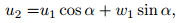
where u0, v0, w0 are the observational data, u1, v1, w1 are the velocities after first rotation. The first rotation has to be performed to align u into the mean wind direction. The second rotation makes x-z plane rotate around y-axis, forcing w=0.
|
(12) |
|
(13) |
|
(14) |

|
(15) |
where u2, v2, w2 are velocities after second rotation. Twice rotations make v2=0, w2=0.
(2) PF
A mean streamline plane is defined on the basis of measurements made in periods long enough to encompass all wind directions. Then u, v, w in time series are rotated to this mean plane. This study selects 1-21 November 2008 except 3 November to determine the plane. The 30 min average of u, v, w are used to compute the equation
set:
|
(16) |

|
(17) |

|
(18) |
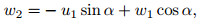
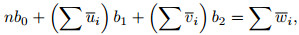
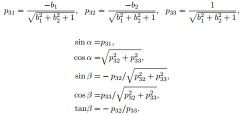
Compute the values of b0, b1, b2 which are used to determine p and rotation angles:
|
(19) |
u, v, w in time series are rotated to this mean plane based on the rotation angles:
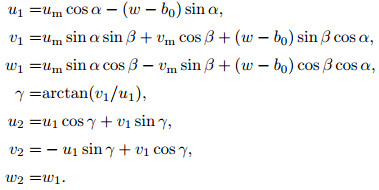
|
(20) |
The WPL correction is necessary because fluctuations in temperature and humidity cause fluctuations in trace gas concentrations that are not associated with the flux of the trace gas we wish to measure. The corrected latent heat flux and CO2 flux are given by
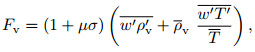
|
(21) |
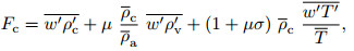
|
(22) |
where µ=1.6 is the ratio of the molecular masses of dry air and water vapor, σ=ρv/ρa is the ratio of the mean densities of water vapor and dry air, ρa is the density of dry air (Webb et al., 1980). WPL is set to add a revised term of heat flux on the latent heat flux, plus revised terms of water vapor and heat flux on CO2 flux.
4 RESULTS AND DISCUSSION 4.1 Sonic Temperature Correction and WPL CorrectionThe results of sonic temperature correction (w'Ts' − w'T')/w'Ts' are shown in Table 1. Sonic temperature correction decreases the sensible heat flux by about 7.3% in DR, while by 5.9% in PF. Liu et al. (2001) have a similar study using LITFASS-1998 experimental data during which the vegetation height is about 0.1 m and vegetation fraction is less than 10%. They have shown the effects of sonic temperature correction being different under stable and unstable conditions that the w'T' is decreased by 10% in stable condition relative to w'Ts', while decreased by 30% under unstable condition. The underlying surface of SACOL in winter is similar to the LITFASS-1998 experiment. In SACOL the w'T' of DR is reduced by 8.5% and w'T' of PF is reduced by 3.5% under stable condition, while w'T' of DR is reduced by 5.5% and w'T' of PF is reduced by 9.4% under unstable condition. Liu et al. (2001) pointed out that the effects of sonic temperature correction are different between stable and unstable conditions and the correction effects are little under stable condition due to limited water vapor content in stable stratification. But our study used the same data including same water vapor content and mean temperature for DR and PF, PF got a similar result with Liu et al., while DR had a contrary result that the effects of correction under stable stratification are stronger than unstable. Therefore, the content of water vapor cannot fully explain the difference of sonic temperature correction under different conditions which may be also related to the vertical velocity of different coordinate rotations.
|
|
Table 1 Comparison of sonic temperature correction of DR and PF |
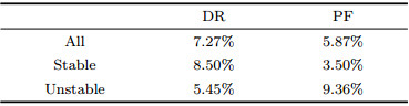
Figure 1 is the daily variations of latent heat flux and CO2 flux before and after WPL correction. The high values of latent heat flux appear at day up to 120 W·m−2, while the value at night is substantially under 5 W·m−2 which is shown in Figs. 1a and 1c. WPL correction increases latent heat flux by 7.4% overall and increases by 5.6% in daytime, whereas decreases by 3.4% in nighttime which is related to the difference of heat transfer direction between day and night. Heat transfer upward makes the density of water vapor at the height of observation reduced during daytime, thus the latent heat flux observed by EC is underestimated, but reversed in nighttime. As shown from Figs. 1b and 1d, downward CO2 flux is highest around midday, while upward CO2 flux is highest around 0:00. Vegetation photosynthesis absorbs atmospheric CO2 forming a downward CO2 flux in daytime and reaches a maximum at midday, while at night vegetation respiration releases CO2 forming a upward CO2 flux in nighttime, thus generates a peak-valley diurnal variation. WPL correction decreases CO2 flux by 72.2% overall and decreases downward CO2 flux and upward CO2 flux by 64.7% and 23.4% in daytime and nighttime, respectively.

|
Fig. 1 WPL correction of latent heat flux (a, c) and CO2 flux (b, d) (1–6 November 2008 except 3rd) |
Figure 2a shows the differences of u*, Fc, LvE and H between original and after sonic temperature correction and WPL correction by DR and PF. Different coordinate rotations have little influence on scalar fluxes Fc, LvE and H, while the values of u* obtained from DR and PF are decreased by 6% and 3% respectively due to excluding the impact of lateral stress caused by instrument tilt. The comparisons of turbulent fluxes between DR and PF are shown in Fig. 2b. As can be seen, H and LvE of DR and PF are very similar, CO2 fluxes of PF are lower than the DR and u* obtained by PF are 6.18% higher than DR, indicating that the three-dimensional wind velocities of two coordinate rotations are quite different.

|
Fig. 2 Comparison of DR and PF fluxes during 1–21 November 2008 (except 3rd) |
As shown in Fig. 3, the wind commonly comes from southeast (SE) and northwest (NW) directions. The flow patterns are different between different wind directions. Therefore, the two wind direction area of 100°~150° and 280°~330° are selected to do planar fit, respectively called FPF.

|
Fig. 3 Frequency distribution of the wind direction during 1-21 November 2008 |
Coordinate rotation aims to make w=0. DR is the average in a certain time period such as 30 min, while PF obtains an average plane in a longer period of time such as several days without requiring the average vertical velocity of short period to be zero. Fig. 4a presents the 30 min average vertical velocity after correction of PF and FPF. It can be seen that the average vertical velocities after PF correction are generally less than the average vertical velocities which are not corrected, but not all zero. The effect of FPF correction on vertical velocity is significantly improved than PF that most of the vertical velocities meet w=0. In complicated terrain such as SOCAL, it is difficult for PF to fit an ideal plane which can have a good correction for each wind direction, respectively. However, FPF which fit planes according to wind direction could better adapt to the actual underlying surface and improve accuracy. PF and FPF have significant difference on momentum but little on scalar fluxes (not shown). The u* obtained by DR, PF and FPF are compared only considering the dominant wind direction 100°~150° and 280°~330° (Figs. 4b, 4c and 4d). The results show that wind direction has no relationship with the correction of u* by DR which reduces u* by 5%. The effects of PF and FPF correction are influenced by the intensity of turbulent exchange and wind direction. As the turbulent exchange strengthened (u* > 0.3 m·s−1), PF and FPF gradually present that the corrected values in SE are bigger than the NW area and fitting effect is better in NW than in SE. Moreover, high values of u* are located in SE regardless which coordinate rotation is used due to the enhanced acceleration caused by topographic uplift from greater difference of terrain height in SE than other directions (Bao, 2012). PF in SE wind area increases u* by 9.23%, yet decreases by 3.86% in the NW area and FPF in SE wind area increases u* by 10.09%, yet decreases by 1.18% in the NW area.

|
Fig. 4 Comparison of three coordinate rotations |
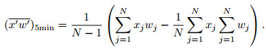
The procedure for stationarity test used in this study was proposed by Foken and Wichura (1996). It compares the statistical parameters determined for the averaging period and for short intervals within this period. In this study the averaging time 30 min will be divided into M=6 intervals of 5 min. There are N=3000 points in each short interval. The covariance of each interval is
|
(23) |
The average covariance of 6 intervals:
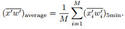
|
(24) |
The covariance of averaging period 30 min:
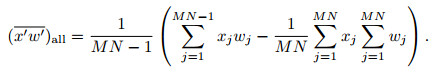
|
(25) |
The time series is in steady state if the difference between both covariances:
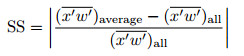
|
(26) |
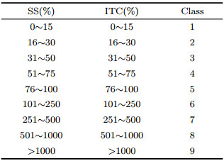
is less than 30%. The values of SS are used to classify the data according to Table 2. Fig. 5 presents the quality classification of stationarity test. Figs. 5a and 5b represent the results of DR and PF, respectively. Whether DR or PF is used, there are 64% of CO2 flux, 74% of latent heat flux and 85% of sensible heat flux classified as good steady state i.e., class 1~3. The differences of the steady state test between DR and PF are mainly in u*(w'u', w'v'). On average, there are 75% of w'u' and 57% of w'v' in DR classified as high quality, while 60% of w'u' and 74% of w'v' in PF. w'u' in DR have better quality of stationarity test than w'v', while w'v' have better quality of stationarity test than w'u' in PF further indicating the sensitivity of u* to coordinate rotations.
|
|
Table 2 Classification of data quality by stationarity test and ITC test |

|
Fig. 5 Frequency distributions of quality level for steady state with different coordinate corrections (a) DR; (b) PF. |
ITC test is developed for testing whether the turbulence is fully developed or not. Monin-Obukhov similarity theory is applicable to fully developed turbulence and normalized dimensionless parameter is the only function of atmospheric stability: 


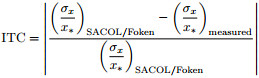
|
|
Table 3 Values of c1 and c2 of different parameterization schemes |
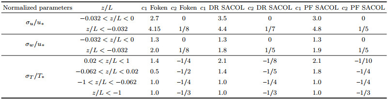
The data with u * < 0.1 m·s−1 when EC is likely unreliable for the turbulent flux measurement are eliminated from analysis of the relationship between normalized dimensionless parameter and stability in SACOL (Zuo et al., 2009). As shown in Fig. 6, the normalized standard deviation of vertical velocity and temperature fit better with stability no matter which coordinate rotation is used. Zhang et al. (2004) considered σw/u* and σT/T* are mainly impacted by local characteristic scale which is relatively small in surface layer, while σu/u* does not entirely depend on local characteristic scale in surface layer. σu/u* is affected by mixed layer scale under strong unstable conditions. Wyngaard and Coté (1971) and Kaimal et al. (1982) also showed that σw/u* can better meet the theory of similarity and are independent of the terrain. This is because that vertical direction consists mainly of small-scale and high frequency eddies which can adapt to the change of terrain quickly, thus the statistics of vertical velocity are less affected by the changing of topography and differences in physical characteristics of underlying. That is to say σw/u* under unstable conditions in complicated underlying of Loess Plateau are similar to the flat underlying and satisfy the theory of similarity well (Moraes, 2000; AJiboori, 2001). The fluctuations of horizontal velocity are mainly produced by large-scale quasi-horizontal turbulence which is a few hundred meters or even larger. The horizontal flow adapts to the terrain slowly and observed horizontal flow always “remembers” the features of upwind terrain producing large variance (Zhao et al., 1991). The relationship between normalized dimensionless parameter and stability of DR and PF in SACOL are shown in Table 3.

|
Fig. 6 Standard deviations of temperature normalized by T*, and horizontal (u), vertical velocity (w) normalized |
ITC derived according to c1, c2 of Foken and SACOL are used to classify data quality as shown in Fig. 7. When using DR coordinate rotation, the quality of u, w, T obtained by SACOL parameterization schemes is significantly improved than Foken scheme by increasing the frequency distribution of high-quality and decreasing frequency distribution of low-quality. When using PF coordinate rotation, the quality of w and T obtained by SACOL parameterization schemes is significantly improved than Foken scheme, but the quality of u has no significant change. SACOL parameterization schemes have a better application on both of the two coordinate rotations. The quality of w is better than u and T in both DR and PF coordinate rotations indicating that the theory of turbulence similarity has a better application on w.

|
Fig. 7 Frequency distributions of quality level for ITC test using different parameterization schemes |
Stationarity test and ITC test aim to filter and select high-quality data to be used for further study. For easy use, Lee et al. (2005) proposed a classification scheme to combine all of the single quality flags given by different tests into a general flag (Table 4). The classes 1~3, classified as high quality, can be used for fundamental research, such as the development of parameterizations; classes 4~6, classified as moderate quality, for general use, such as long term observation programs; and classes 7~9, classified as low quality, should be excluded from further analysis or replaced by gap-filling.
|
|
Table 4 Overall quality classification |

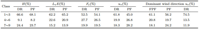
Table 5 shows the overall quality distribution of turbulent fluxes corrected by DR, PF and FPF, respectively. The overall quality shows that about 66%~68% of the total data are of high quality for sensible heat flux, 62%~65% for latent heat flux and 52%~54% for CO2 flux. Coordinate rotations have little effect on these three scalar fluxes. The proportion of high quality data of these three fluxes obtained by PF is 2%~3% higher than DR. While the overall quality shows that only about 45% of the total data are of high quality for u* after PF correction which is consistent with the results of Zuo et al. (2009) that the quality of u* is low under complicated terrain and need to be further improved. After DR correction, about 62% of the total data are of high quality for u* which is 17% higher than PF. In order to compare with FPF, the data in dominant wind direction are selected for further analysis. It is worth noting that all wind direction data are used to determine the angle of rotation in DR and PF. The prevailing wind direction is still dominant in determining the angle of rotation even with the impact of non-dominant wind direction. So when excluding non-dominant wind direction, the quality of u* from PF and DR is also improved. After FPF rotation, about 61% of the total data are of high quality for which is significantly improved compared with PF, but the quality of after DR rotation is still the highest. Wilczak et al. (2001) pointed out that the sampling error of the mean vertical velocity results in a tilt angle estimation error in DR. This adds a random noise component to the longitudinal stress estimate, making the stress more uncertain. In PF rotation many data are used to determine the PF tilt angle which is much less susceptible to sampling errors. Zhu et al. (2004) considered that PF is not suitable for complicated terrain. This study considers that the use of DR is recommended in the complicated terrain for reducing calculation and improving the data quality.
|
|
Table 5 Overall quality of H, LvE, Fc and u* using different coordinate rotations |
Turbulent data from SACOL are used to analyze the applicability of DR, PF and FPF over complicated terrain. The data processing and quality control including sonic temperature correction, coordinate rotations, WPL correction, stationarity test and ITC test effectively reduce the additional error of turbulence observational data due to terrain and improve data quality.
(1) Sonic temperature correction decreases sensible heat flux by about 7.3% when using DR, but 5.9% when using PF. The stability would influence the results of sonic temperature correction. WPL increases latent heat flux by 7.4% and decreases CO2 flux by 72.2%.
(2) The values of u* obtained from DR and PF are decreased by 6% and 3% respectively. Only considering the dominant wind direction, the wind direction has no relationship with the correction of u* by DR which reduces u* by 5%. As the turbulent exchange strengthened (u* > 0.3 m·s−1), PF and FPF gradually present that the corrected values in SE are bigger than the NW area, PF in SE wind area increases u* by 9.23%, yet decreases by 3.86% in the NW area and FPF in SE wind area increases u* by 10.09%, yet decreases by 1.18% in the NW area.
(3) A parameterization scheme for SACOL provided in ITC test applies well in both DR and PF.
(4) The proportion of the high quality u* obtained by DR is 17% higher than by PF, while the proportion of high quality data of sensible heat, latent heat and CO2 flux obtained by PF is 2%~3% higher than DR. The differences between PF and FPF are mainly in u*. Comparing the three coordinate rotations in the dominant wind direction, DR still obtains the best quality of u*. The use of DR is recommended in the complicated terrain for reducing calculation and improving the data quality.
ACKNOWLEDGMENTSThe research is supported by the National Natural Science Foundation of China (41475008) and the National Basic Research Program of China (2012CB955302). The authors would like to thank the Semi-Arid Climate and Environment Observatory of Lanzhou University (SACOL) for providing observational data. We would also like to thank the anonymous reviewers for their critical and helpful comments and suggestions.
| [] | Al-Jiboori M H, Xu Y M, Qian Y F. 2001. Turbulence characteristics over complex terrain in west China. Boundary-Layer Meteorology , 101 (1) : 109-126. DOI:10.1023/A:1019234724291 |
| [] | Aubinet M, Vesala T, Papale D. 2011. Eddy Covariance:A Practical Guide to Measurement and Data Analysis. New York:Springer. |
| [] | Baldocchi D, Falge L, Gu L H, et al. 2001. FLUXNET:A new tool to study the temporal and spatial variability of ecosystem-scale carbon dioxide, water vapor, and energy flux densities. Bull. Amer. Meteor. Soc. , 82 (11) : 2415-2434. DOI:10.1175/1520-0477(2001)082<2415:FANTTS>2.3.CO;2 |
| [] | Bao J. 2012. Study on land-atmosphere interaction in surface layer over semi-arid Loess Plateau of China[Ph. D. thesis](in Chinese). Lanzhou:Lanzhou University. |
| [] | Chen Z G, Bian L G, Lu L H, et al. 2008. Contrast and application of tilt correction methods for eddy covariance measurement. Meteor. Sci. Technol. (in Chinese) , 36 (3) : 355-359. |
| [] | Ding Y H. 1997. On some aspects of estimates of the surface fluxes. Quarterly Journal of Applied Meteorology (in Chinese) , 8 (S) : 29-35. |
| [] | Foken T, Wichura B. 1996. Tools for quality assessment of surface-based flux measurements. Agricultural and Forest Meteorology , 78 (1-2) : 83-105. DOI:10.1016/0168-1923(95)02248-1 |
| [] | Foken T. 2008. The energy balance closure problem:An overview. Ecol. Appl. , 18 (6) : 1351-1367. DOI:10.1890/06-0922.1 |
| [] | Göckede M, Foken T, Aubinet M, et al. 2008. Quality control of CarboEurope flux data-Part 1:Coupling footprint analyses with flux data quality assessment to evaluate sites in forest ecosystems. Biogeosciences , 5 (2) : 433-450. DOI:10.5194/bg-5-433-2008 |
| [] | Huang J P, Zhang W, Zuo J Q, et al. 2008. An overview of the semi-arid climate and environment research observatory over the loess plateau. Adv. Atmos. Sci. , 25 (6) : 906-921. DOI:10.1007/s00376-008-0906-7 |
| [] | Jiang H M, Liu S H, Liu H P. 2012. A study on energy budget characteristics over a heterogeneously irrigated cotton field. Chinese J. Geophys. (in Chinese) , 55 (2) : 428-440. DOI:10.6038/j.issn.0001-5733.2012.02.007 |
| [] | Jiang H M, Liu S H, Zhang L, et al. 2013. A study of turbulent heat flux corrections and energy balance closure problem on the surface layer in EBEX-2000. Acta Scientiarum Naturalium Universitatis Pekinensis (in Chinese) , 49 (3) : 443-451. |
| [] | Jiang H M, Liu S H, Liu H P. 2013. Spectra and cospectra of turbulence in an internal boundary layer over a heterogeneously irrigated cotton field. Acta Meteor. Sin. , 27 (2) : 233-248. DOI:10.1007/s13351-013-0208-6 |
| [] | Kaimal J C, Finnigan J J. 1994. Atmospheric Boundary Layer Flows:Their Structure and Measurement. Oxford:Oxford University Press. |
| [] | Kaimal J C, Eversole R A, Lenschow D H, et al. 1982. Spectral characteristics of the convective boundary layer over uneven terrain. J. Atmos. Sci. , 39 (5) : 1098-1114. DOI:10.1175/1520-0469(1982)039<1098:SCOTCB>2.0.CO;2 |
| [] | Lee X H, Massman W, Law B. 2005. Handbook of Micrometeorology:A Guide for Surface Flux Measurement and Analysis. Netherlands:Springer. |
| [] | Liang J N, Zhang L, Tian P F, et al. 2014. Impact of low-level jets on turbulent in nocturnal boundary layer over complex terrain of the Loess Plateau. Chinese J. Geophys. (in Chinese) , 57 (5) : 1387-1398. DOI:10.6038/cjg20140504 |
| [] | Liu H P, Peters G, Foken T. 2001. New equations for sonic temperature variance and buoyancy heat flux with an omnidirectional sonic anemometer. Boundary-Layer Meteorology , 100 (3) : 459-468. DOI:10.1023/A:1019207031397 |
| [] | Liu S H, Li J, Liu H P, et al. 2005a. Characteristics of macroturbulence variables in EBEX-2000. Chin. J. Atmos. Sci.(in Chinese) , 29 (4) : 503-509. |
| [] | Liu S H, Liu H P, Li J, et al. 2005b. Characteristics of turbulence dissipation rates, characteristic length scales and structure parameters in EBEX-2000. Chin. J. Atmos. Sci. (in Chinese) , 29 (3) : 475-481. |
| [] | Liu S H, Hu Y, Hu F, et al. 2005c. Numerical simulation of land-atmosphere interaction and oasis effect over oasis-desert. Chinese J. Geophys. (in Chinese) , 48 (5) : 1019-1027. DOI:10.3321/j.issn:0001-5733.2005.05.007 |
| [] | Liu S H, Mao Y H, Hu F, et al. 2009. A comparative study of computing methods of turbulent fluxes on different underling surfaces. Chinese J. Geophys. (in Chinese) , 52 (3) : 616-629. |
| [] | Mauder M, Liebethal C, Gckede M, et al. 2006. Processing and quality control of flux data during LITFASS-2003. Boundary-Layer Meteorology , 122 (1) : 67-88. |
| [] | Moraes O L L. 2000. Turbulence characteristics in the surface boundary layer over the South American Pampa. Boundary-Layer Meteorology , 96 (3) : 317-335. DOI:10.1023/A:1002604624749 |
| [] | Schotanus P, Nieuwstadt F T M, De Bruin H A R. 1983. Temperature measurement with a sonic anemometer and its application to heat and moisture fluxes. Boundary-Layer Meteorology , 26 (1) : 81-93. DOI:10.1007/BF00164332 |
| [] | Swinbank W C. 1951. The measurement of vertical transfer of heat and water vapor by eddies in the lower atmosphere. J. Meteor. , 8 (3) : 135-145. DOI:10.1175/1520-0469(1951)008<0135:TMOVTO>2.0.CO;2 |
| [] | Vickers D, Mahrt L. 1997. Quality control and flux sampling problems for tower and aircraft data. J. Atmos. Oceanic. Technol. , 14 (3) : 512-526. DOI:10.1175/1520-0426(1997)014<0512:QCAFSP>2.0.CO;2 |
| [] | Wang J M, Wang W Z, Ao Y H, et al. 2007. Turbulence flux measurements under complicated conditions. Adv. Earth Sci. (in Chinese) , 22 (8) : 791-797. DOI:10.3321/j.issn:1001-8166.2007.08.004 |
| [] | Wang S Y, Zhang Y, Lü S H, et al. 2009. The preliminary study on turbulence data quality control of Jinta oasis. Plateau Meteorology (in Chinese) , 28 (6) : 1260-1273. |
| [] | Webb E K, Pearman G I, Leuning R. 1980. Correction of flux measurements for density effects due to heat and water vapour transfer. Quart. J. Roy. Meteor. Soc. , 106 (447) : 85-100. DOI:10.1002/(ISSN)1477-870X |
| [] | Wilczak J M, Oncley S P, Stage S A. 2001. Sonic anemometer tilt correction algorithms. Boundary-Layer Meteorology , 99 (1) : 127-150. DOI:10.1023/A:1018966204465 |
| [] | Wyngaard J C, Coté O R. 1971. The budgets of turbulent kinetic energy and temperature variance in the atmospheric surface layer. J. Atmos. Sci. , 28 (2) : 190-201. DOI:10.1175/1520-0469(1971)028<0190:TBOTKE>2.0.CO;2 |
| [] | Xu Z W, Liu S M, Gong L J, et al. 2008. A study on the data processing and quality assessment of the eddy covariance system. Adv. Earth Sci. (in Chinese) , 23 (4) : 357-370. DOI:10.3321/j.issn:1001-8166.2008.04.005 |
| [] | Yang W Z, Shao M A. 2000. The Research of the Loess Plateau Soil Moisture (in Chinese)[M]. Beijing: Science Press . |
| [] | Zhang H S, Li F Y, Chen J Y. 2004. Statistical characteristics of atmospheric turbulence in different underlying surface conditions. Plateau Meteorology (in Chinese) , 23 (5) : 598-604. |
| [] | Zhao M, Miao M Q, Wang Y C. 1991. Boundary-Layer Meteorology (in Chinese)[M]. Beijing: China Meteorological Press . |
| [] | Zhu Z L, Sun X M, Yuan G F, et al. 2004. Correcting method of eddy covariance fluxes over non-flat surfaces and its application in China FLUX. Sci. China Ser. D:Earth Sci. , 48 (S1) : 42-50. |
| [] | Zuo J Q, Huang J P, Wang J M, et al. 2009. Surface turbulent flux measurements over the loess plateau for a semi-arid climate change study. Adv. Atmos. Sci. , 26 (4) : 679-691. DOI:10.1007/s00376-009-8188-2 |