 2016, Vol. 59


Complex reservoirs have been research hotspots in recent years, due to the increasing demand for oil and gas resources, as well as the in-depth study of the development and exploration of oil and gas fields. Of those, the reservoir evaluations of volcanic clastic rock and volcanic clastic sedimentary reservoirs have drawn wide attention. However, the research level has not yet been deep enough (Zhang et al., 2013; Liu et al., 2014).
Tuffaceous sandstone is a type of common volcaniclastic sedimentary rock. To date, the studies regarding the logging interpretation of the tuffaceous sandstone reservoirs have been inadequate, and the available infor mation has been very limited. In 1973, Khatchikian et al. proposed a method of log interpretation for tuffaceous reservoirs in southern Argentina, which used sonic, density, and neutron logs to calculate the shale and tuff content. A model of the shale-sand was used to calculate the porosity and water saturation (Khatchikian et al., 1973). However, a wide use of this method was difficult to achieve, due to the lack of pertinent details for the theory and algorithm. Itoh et al. (1982), without experimental verification, assumed that the tuff also had some electric conductance similar to that of the shale. Furthermore, a method of calculating the saturation level of the volcanic tuff using the cation exchange capacity (CEC) was proposed. This method was mainly used for tuffaceous reservoirs (Itoh et al., 1982). In 2006, Xiao evaluated the tuffaceous sandstone reservoirs of the Xing’anling Group in Hailar Basin, and a method of calculating the saturation using HB and S-B models was proposed. However, it was found that there was an instability in the calculation of the cementation exponent of the clay matrix with the HB resistivity model. Also, the S-B model was determined to be suitable for reservoirs with high tuff (Xiao, 2006).
The present study took tuffaceous sandstone reservoirs with the same source of tuff in the X Depression of the Hailar-Tamtsag Basin as an example. The component content was calculated using a method which combined a bacterial foraging algorithm, and a particle swarm optimization algorithm. The electrical conductivity of the tuff was proven using CEC experimental data. The CEC ratio was used to calculate the water saturation of the tuffaceous sandstone reservoirs, and the results of the application were found to be encouraging.
2 CALCULATION OF THE TUFF CONTENT USING A HYBRID OPTIMIZATION ALGORITHM 2.1 Reservoir Physical PropertyIn this study, volcaniclastic and volcaniclastic sedimentary rocks were found to be common reservoir rock types in the X Depression of the Hailar-Tamtsag Basin. Tuffaceous sandstone is one of the typical volcaniclastic sedimentary rocks. This type of reservoir, which has small development thickness, uneven particle size distribution, and complex mineral composition, is difficult to identify with conventional well-logging data. The tuff had a large variation range, but the variation range of the shale content was smaller. The distribution of the shale content was mainly concentrated in 5% to 25% of the study area. The reservoirs contained tuff, which caused significant variations in the reservoirs’ pore structures, physical properties, aeolotropism, and well-logging curves. Also, these characteristics led to great differences in the well-logging responses, which increased the difficulty of the evaluations. The porosity of reservoirs in the study area was mainly concentrated in the 5% to 20% range, and the permeability range was (0.01~120)×10−3 µm2.
2.2 Calculation of the Logging Response Values of the Reservoir ComponentsThe calculation of the logging response values of the reservoir components was a precondition for the quantitative determination of the shale content, as well as other content. Xiao divided the tuffaceous sandstone reservoirs into four parts: shale, tuff, sandstone matrix, and pore. Fig. 1 shows the volume model of the tuffaceous sandstone reservoir proposed by Xiao.

|
Fig. 1 Volume model of the tuffaceous sandstone reservoir |
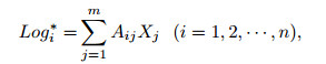
Fifteen tuffaceous sandstone rock samples from the X Depression of the Hailar-Tamtsag Basin were used to calculate the logging response values of the reservoir components using a Quasi Newton algorithm. Then, based on the volume model and logging response differences between the shale and tuff, the log response equation (Formula (1)) and objective function (Formula (2)) were established as follows:
|
(1) |
|
(2) |
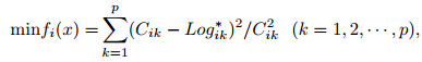
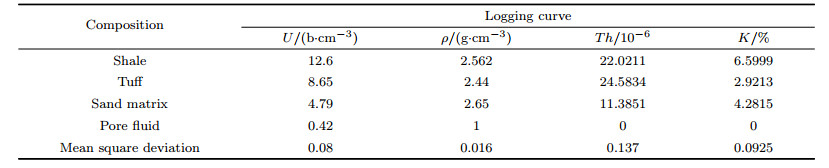
where Logi* is the calculated value of the ith log response; Xj is the content of the jth formation component; and Aij is the ith log response value of the jth formation component. Formula (2) is the objective function of ith log response, and Cik is the ith log response value of the kth rock sample. The photoelectric absorption cross-section index per unit volume of the rock (U), density (ρ), thorium (Th), and potassium (K) logs are chosen for the analyses. The U and ρ of the sandstone matrix were theoretical values. It was assumed that the pore fluid did not contain radioactive elements. Table 1 lists the logging response values of the formation components, and the mean square deviations were less than 0.15.
|
|
Table 1 Logging response values of the formation components |
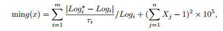
Particle swarm optimization (PSO) is a type of community intelligent optimization methods. The PSO has a large number of characteristics, such as simple structure, few parameters, and fast convergence rate, which can be used to process large amounts of logging data. The possible solutions of the components can be used to calculate the current fitness value using objective function (3), in order for the particle with the best fitness to be found. In each iteration, the velocity and position of the particles will be updated as follows:
|
(3) |
where Logi* is the calculated value of the ith log response; Logi is the measured value of the ith log response; and Xj is the content of the jth formation component. Although the PSO is simple, fast, and easy to calculate, it is also easy to fall into local optimal problems.
The bacterial foraging algorithm (BFA) is the optimization of searching for the state of bacteria in space, which is based on the simulation of the foraging behavior of Escherichia coli in human intestinal tracts. The foraging behavior of bacteria includes three patterns: chemotaxis, reproduction, and copying (Yang et al., 2012). During a chemotactic process, the foraging pattern of bacteria mainly includes turning and advancing (You et al., 2013). If the fitness is improved after a turnover, the bacteria will continue to move in the same direction until the fitness value is no longer improving. During a chemotactic process, the position of the bacteria will be updated as follows:

|
(4) |
where θi(j, k, l) is the position of the ith bacteria in the jth chemotactic process; C is the step length of the chemotaxis; and ∠ϕ is the angle of the turnover.
Once the bacteria are unable to obtain enough food, that is, the bacteria enter into a critical chemotactic period, half of the bacteria will die, and half will continue to breed in order to maintain a foraging capacity. Following propagation, some of the bacteria will be dispersed to other locations, and the other bacteria will remain unchanged in their position. Migration operations are able to improve global search abilities, as well as enhance the ability of the bacteria to jump out of a local optimal solution (You et al., 2013). The advantage of a bacterial foraging algorithm is in the search of a global optimal solution. However, the convergence rate is slow. Although a BFA is able to obtain a global optimal solution, it has slow convergence rate.
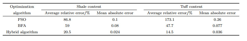
PSO has high calculation speed, but it is easy to fall into local optimal problems. The BFA is able to find global optimal solutions, but has slow convergence rate. Therefore, a method which combined bacterial foraging and particle swarm optimization algorithms was proposed in this study. The hybrid optimization algorithm improved the calculation accuracy, which integrated the advantages of both PSO and BFA (Yang et al., 2012; Tan et al., 2012; Pan et al., 2016). In this study, this hybrid optimization algorithm was applied to evaluate the reservoir. Table 2 lists the calculation results using three optimization algorithms: PSO, BFA, and hybrid algorithm. The results of the hybrid algorithm were found to be better than that of the PSO and BFA, which proved the feasibility of the method.
|
|
Table 2 Calculation results using three optimization algorithms |
Itoh (1982) assumed that tuff and shale have similar electrical conductivity (Itoh et al., 1982). Although this assumption is widely recognized (Zhang et al., 2009; Xiao, 2006), there is still no experimental evidence to support it. This study used the experimental data of cation exchange capacity (CEC) to prove that tuff has electrical conductivity.
The cation exchange capacity is able to reflect the additional conductivity of rock. The higher the CEC value is, the greater the additional conductivity of the rock will be. Due to the presence of shale and tuff in the tuffaceous sandstone, this study assumed that the CEC only originated from the shale and tuff. In order to remove the influence of the shale, samples with the same shale content were used to analyze the relationship between the tuff content and the CEC level. The data used in this study included the thin section analysis data, X-ray diffraction based whole-rock quantitative analysis data, and the shale and tuff content of 63 rock samples in the study area, of which 62 rock samples had their CEC value determined. Fig. 2 presents the relationship between the tuff content and CEC value of eight rock samples with the same shale content. It can be seen from the figure that tuff content was in positive correlation with the CEC level, which proved that the tuff had electrical conductivity.

|
Fig. 2 Relationship between the samples’ CEC and tuff contents for shale content 0.12 |
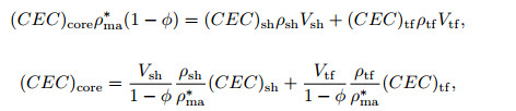
In this study it was assumed that the CEC only originated from the shale and tuff, and the CEC value of the sandstone was 0. The equation of the material balance was as follows:

|
or
|
(5) |
where ρma* is the particle density of tuffaceous sandstone; (CEC)tf is the CEC value of the tuff, in mmol/100 g; (CEC)sh is the CEC value of the shale, in mmol/100 g; and ρsh and ρtf represent the density of shale and tuff, respectively, in g·cm−3.
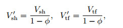
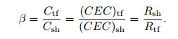
The two parameters were defined as follows:
|
(6) |
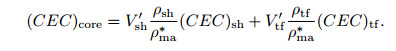
where V'sh and V'tf represent the content of the shale and tuff, respectively, corrected for porosity. By combining Formulas (5) and (6), Formula (7) was achieved as follows:
|
(7) |
Due to the fact that 


|
Fig. 3 Relationship between CEC of tuffaceous sandstone and V'th with V'sh in [0.18, 0.2] |
Based on the above, this study calculated the ρ × CEC and CEC ratios between the shale and tuff as follows:
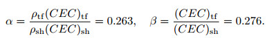
|
Itoh et al. calculated the CEC ratio between the shale and tuff using Formula (7). When V'sh=0, Itoh et al. set the V'tf to be the value of (CEC)core. Also, they took V'sh to be the value of (CEC)core when V'tf=0. Therefore, the CEC ratio calculated by Itoh et al. was actually the ρ × CEC ratio. Through the analysis of the CEC data, it was found that the tuff not only had a cation exchange capacity, but also the capacity was weaker than that of the shale.
3.2 Calculation of the Water Saturation Using a CEC Ratio MethodFigure 1 shows the volume model of the tuffaceous sandstone reservoir in the study area. In the figure, the side length of the volume model is L; the cross-section area is S; the cross-section area of the tuff is Stf; and its relative volume is Vtf. The cross-section area of the shale is Ssh, and its relative volume is Vsh. The cross-section area of the sand is Ssd, and its relative volume is Vsd. The side lengths of the shale, tuff, and sand are all L, and φ is the total porosity. It was assumed that the current flowed to the formation in a direction which was perpendicular to the cross-section of the rock. Therefore, the tuffaceous sandstone could be treated as the parallel conduction between the tuff, shale, and sandstone, as shown in Fig. 4 (Xiao, 2006).

|
Fig. 4 Equivalent circuit of the tuffaceous sandstone |
Therefore, the resistance of the tuffaceous sand stone was expressed as follows:
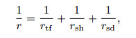
|
(8) |
where rtf, rsh and rsd are the resistance of tuff, shale, and sandstone, respectively. Rt, Rtf, Rsh and Rsd are the resistivity of the rock, tuff, shale, and sandstone, respectively.
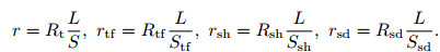
|
(9) |
When Eq.(9) is put into Eq.(8), Eq.(10) could be reformed as follows:
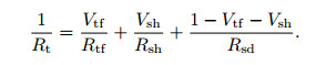
|
(10) |
The Archie formula was applied to the pure sandstone, and the water saturation could be expressed as follows:
|
(11) |
where SW is the water saturation; RW is the formation water resistivity, in Ω·m; a is the factor in relation to the rock; b is a constant related to the lithology; m is the cementation factor; and n is the saturation index.
In this study, when the resistivity of the tuff was unavailable, the CEC data were used to calculate the water saturation. Waxman and Smits (1968) proposed conductivity models for shale sand formations as follows:
|
(12) |
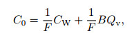
where 
|
(13) |
where C0 and CW are the conductivity of the formation water and shale sand with 100% water respectively, in S·m−1; Csh is the additional conductivity induced by the shale, in S·m−1; F is the formation factor of the shale sand; B is the equivalent electrical conductance of the exchangeable cations, in S·cm3/(mmol·m); and Qv is the cation exchange capacity, in mmol·cm−3, which can be expressed as follows:
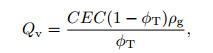
|
(14) |
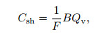
where ρg is the particle density, g·cm−3; and φT is the total porosity. When Eq.(14) was put into Eq.(13) with the application of (CEC)sh instead of CEC, Eq.(15) could be reformed as follows:
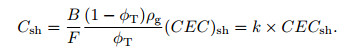
|
(15) |
The Csh values showed a linear correlation to the CEC of shale, as shown in Formula (15). Therefore, the values were also linearly associated with (CEC)tf as follows:

|
(16) |
where k in Formula (16) is the same as in Formula (15):
|
(17) |
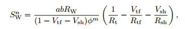
When Eq.(17) was input into Eq.(11), the water saturation could be expressed as follows:
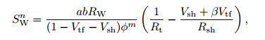
|
(18) |
where the values of a, b, m and n were obtained from the rock electric experiment; and φ equals the average of the calculation of the two methods: hybrid optimization algorithm and neutron-density cross-plot. The value of Rsh equals the resistivity of the thick shale layer adjacent to the target intervals; and RW is calculated with the use of the salinity of the formation water, reservoir depth, temperature, and so on. The calculation of β was as mentioned above. In this study, the Vsh and Vtf were obtained using the hybrid optimization algorithm. The method was proposed to calculate the water saturation, and is referred to as the CEC ratio method.
4 APPLICATION EXAMPLEThe a, b, m and n mentioned above were the key parameters in the calculation of the water saturation, which changed with the geological conditions. Therefore, the electrical rock experiment which was used to calculate a, b, m and n was the basis for evaluation of water saturation in the study area. A displacement experiment under the reservoir conditions had been done in the study area. However, it had not been applied to the calculation of the water saturation (Wang et al., 2012). 31 rock samples were tested under the reservoir conditions, of which 18 rock samples were sandstone, and the remainder were tuffaceous sandstone.
Figure 5 presents the relationship between the formation factors and the porosities of the tuffaceous sandstone. The solid and dashed lines represent the trend line of the formation factors vs. the porosities in the sandstone and tuffaceous sandstone, respectively. For the sandstone, a=1.354 and m=1.784 were obtained. For the tuffaceous sandstone, a=1.149 and m=1.919 were obtained.

|
Fig. 5 Relationship between formation factors and porosities of tuffaceous sandstone in reservoirs |
Figure 6 illustrates the relationship between the resistivity indexes (I) and the water saturation (SW) under the reservoir conditions. The solid and dashed lines represent the trend line of I vs. SW in the sandstone and tuffaceous sandstone, respectively. For the sandstone, b=0.966 and n=1.596 were obtained. For the tuffaceous sandstone, b=0.983 and n=1.86 were obtained.

|
Fig. 6 Relationship between resistance increments and water saturations of tuffaceous sandstone in reservoirs |
Three tuffaceous sandstone reservoir intervals from three wells in the study area were selected for the logging evaluation, using the above method along with an Archie formula. Fig. 7 shows the log interpretation of the three reservoir intervals. When the CEC ratio method was used to evaluate saturation, the values of a, b, m and n for sandstone were calculated. The values of a, b, m and n for the tuffaceous sandstone were then applied to an Archie formula. Since the data of sealed coring and oil testing were limited, only three intervals (levels A, B, and C) were selected for the evaluation.

|
Fig. 7 Log interpretation of the tuffaceous sandstone reservoir (levels A, B, and C) in the X Depression of the Hailar-Tamtsag Basin |
In Fig. 7, Vtf- 1 and Vsh- 1 represent the tuff and shale content, respectively, using a thin section analysis. POR core is the porosity from the core analysis data; SW is the saturation calculated using the CEC ratio method; SW- Archie is the saturation calculated with the Archie formula; SWI is the irreducible water saturation which was calculated using the relationship between the porosity and the irreducible water saturation from the core NMR data. It can be seen that the calculated content of the shale and tuff had high consistency with the section analysis data. The calculated value of SW correspondeds to the test oil conclusion and SWI at the A and B layers. Meanwhile, the calculated value of SW- Archie was significantly larger than the SWI. The calculated values of SW and SW- Archie were both larger than the SWI at the C layer, which corresponded to the conclusions of the oil testing. When compared with the Archie formula, the calculation method of the saturation for tuffaceous sandstone reservoir proposed in this study proved to be more effective in the identification of the oil layers.
5 CONCLUSIONSThe distinction of shale and tuff, along with the calculations of their content, are difficult problems in the logging evaluation of tuffaceous sandstone reservoirs. Therefore, based on the differences in the log response characteristics between tuff and shale, a hybrid optimization algorithm was preferentially selected for the calculation of tuff content in this study. Also, the calculated content of the tuff was found to have a high consistency with the section analysis data. This study used CEC data to prove that the tuff had an electric conductance which was similar to that of the shale, and the tuff was able to produce additional conductivity. The relationship between the CEC and resistivity was obtained based on a W-S model. Furthermore, a new method for calculating the water saturation was proposed. A log evaluation was performed with intervals from three wells in the X Depression of the Hailar-Tamtsag Basin. When compared with the Archie formula, the CEC ratio method proposed in this study achieved good results.
| [] | Itoh T, Kato S, Miyairi M. 1982. A quick method of log interpretation for very low resistivity volcanic tuff by the use of CEC data//Proceedings of the 23rd SPWLA Annual Logging Symposium. Corpus Christi, Texas. |
| [] | Khatchikian A, Lesta P. 1973. Log evaluation of tuffites and tuffaceous sandstones in Southern Argentina//Proceedings of the SPWLA 14th Annual Logging Symposium. Lafayette, Louisiana. |
| [] | Liu S H, Pan B Z, Huang B Z, et al. 2014. The review on the evaluation methods of Volcani-clastic sedimentary rock reservoirs. Progress in Geophysics (in Chinese) , 29 (2) : 798-804. DOI:10.6038/pg20140244 |
| [] | Liu X L, Zhao K L. 2011. Bacteria foraging optimization algorithm based on immune algorithm. Journal of Computer Applications (in Chinese) , 32 (3) : 634-637. |
| [] | Pan B Z, Duan Y N, Zhang H T, et al. 2016. BFA-CM optimization log interpretation method. Chinese J. Geophys. (in Chinese) , 59 (1) : 391-398. DOI:10.6038/cjg20160133 |
| [] | Tan M J, Zou Y L. 2012. A hybrid inversion method of (T2, D) 2D NMR logging and observation parameters effects. Chinese J. Geophys. (in Chinese) , 55 (2) : 683-692. DOI:10.3969/j.issn.0001-5733.2012.02.032 |
| [] | Wang F, Pan B Z, Xiao L, et al. 2012. An experiment comparing electrical parameters of volcani-clastic sedimentary rock and analysis of influence factors. World Well Logging Technology (in Chinese) (4) : 23-25, 34. |
| [] | Waxman W H, Smits L J M. 1968. Electrical conductivities in oil bearing shaly sands. Society of Petroleum Engineers. SPE 1863-A. |
| [] | Xiao D S. 2006. Interpretation method study on physical property of the tuffaceous sands reservoir of Xing'anling Group in Hailar Basin[master's thesis] (in Chinese). Daqing:Daqing Petroleum Institute. |
| [] | Xu H. 2013. Research on particle swarm optimization algorithm improvement and application in CBM production forecast[Ph. D. thesis] (in Chinese). Xuzhou:China University of Mining & Technology. |
| [] | Yang P, Sun Y M, Liu X L, et al. 2011. Particle swarm optimization based on chemotaxis operation of bacterial foraging algorithm. Application Research of Computers (in Chinese) , 28 (10) : 3640-3642. |
| [] | Yang S J, Wang S W, Tao J, et al. 2012. Multi-objective optimization method based on hybrid swarm intelligence algorithm. Computer Simulation (in Chinese) (6) : 218-222. |
| [] | You M L, Lei X J. 2013. An improved bacterial foraging algorithm for the traveling salesman problem. Journal of Guangxi University (Natural Science Edition) (in Chinese) , 38 (6) : 1436-1443. |
| [] | Zhang L H, Pan B Z, Shan G Y. 2013. On comprehensive log evaluation method of volcanic reservoir. Well Logging Technology (in Chinese) , 37 (1) : 53-58. |
| [] | Zhang X F, Pan B Z, Fan X M, et al. 2009. Computational method of saturation of the tuffaceous sandstones reservoir of Nantun Group in Hailar Basin. Well Logging Technology (in Chinese) , 33 (4) : 345-349. |