 2016, Vol. 59


The ionosphere is an important part of the terrestrial space, in which the propagation of radio wave can be influenced and a variety of effects can be caused. The radio communication quality is determined by the state of the ionosphere to a large extent. People has been concerned about the solar activity, the physical processes of magnetosphere and other natural phenomena which can lead to the ionospheric disturbances, at the same time, the artificial modification of the ionosphere is paid more and more attention. It has been observed that the electron heating is followed by expulsion of the plasma from the heated region (Duncan et al., 1988). Numerous observations show that strong electron heating in the ionosphere can be generated by powerful HF facilities such as HAARP and EISCAT (Papadopoulos et al., 2003, 2005).
In the aspect of the theoretical study of ionospheric heating, domestic and foreign scholars have done a lot of work. Huang et al. (2003) established the heating model of ionospheric F region. Fang et al. (2012) calculated the effects of HF heating at the F layer, the electron temperature and density perturbation in the range of 150~500 km is given under different heating conditions. Perrine et al. (2006) used an ionospheric numerical model to study the effects of localized HF heating on an interhemispheric magnetic flux tube. Milikh et al.(2008, 2010, 2012) compared the heating effects from SAMI2 with the satellite data, the results showed that they are in good agreement. Due to the adoption of dipole field coordinates in SAMI2 mode, heating simulation can give the electron temperature and density perturbation results along the whole field line, which provides basis for understanding the ionospheric heating effect comprehensively.
This article is organized as follows. In Section 2 we describe the ionospheric heating model. The heating term (QHF) is added to the electron temperature equation in SAMI2. In Section 3, the procedures and parameters are given. Accounting for the effect of self-action, then the numerical simulation results of high-power HF artificial heating is presented in Section 4. In Section 5, we summarize our conclusions, and also discuss our results and the limitations of this study.
2 SAMI2 IONOSPHERIC HEATING MODELThe ionospheric model SAMI2 (Sami2 is Another Model of the Ionosphere) was developed by the Naval Research Laboratory (Huba et al., 2000). The code is an Eulerian grid-based code, which describes the ionosphere made up of seven ion species: H+, He+, O+, O2+, N+, N2+, NO+. The equations of continuity and momentum are solved for the electrons and each ion species, with the temperature equation solved for the electrons and the species H+, He+, O+. Electron density is calculated by summing the densities of each species, as quasi-neutrality is assumed everywhere in the plasma. The code includes ion chemistry models, horizontal winds, ion inertia, photo-deposition into the ionosphere, a neutral atmosphere model, and E × B drift of the field lines (in altitude and longitude)(Huba et al., 2000).
The SAMI2 model is inter-hemispheric and can thus simulate the plasma along entire magnetic dipole field lines, from the topside magnetosphere down to nearly the E layer (Milikh et al., 2012). Neutral species parameters are provided by the empirical model of NRLMSIS-00 (Mass Spectrometer Incoherent Scatter) model (Picone et al., 2002), with the neutral wind parameters are given by HWM93 (the Horizontal Wind) model (Hedin et al., 1991).
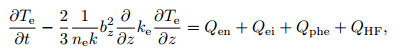
In the original code of SAMI2, three heating terms are included in the electron temperature equation, they are electron-neutral collisions, Qen, electron-ion collisions, Qei and photoelectron heating, Qphe. In this paper, a fourth electron heating term, QHF, has been added to the electron temperature equation in SAMI2, then the electron temperature equation is written as (Perrine et al., 2006)
|
(1) |
where k is the Boltzmann constant, ke is the parallel electron thermal conductivity, bz is the component of the magnetic field in the direction of the field line, normalized to its equatorial value on Earth’s surface. Qphe, Qei and Qen are defined in detail by Huba et al. (2000).
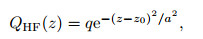
QHF is regarded as Gauss distribution (Perrine et al., 2006), the expression is
|
(2) |
where QHF is the total heating rate per electron (unit: K·s−1), q is the heating rate per electron (unit: K·s−1), z0 is the height of the heated spot’s center (unit: km), a the vertical extent of the heated region (unit: km).
3 PROCEDURES AND PARAMETERSFor simplicity, we ignore the E × B drift of the plasma. Two numerical experiments are designed in this paper, which are described as follows:
Experiment Ⅰ: The code starts at 10:00 LT (local time), and runs for 12 hours without HF heating. This allows the system to relax to ambient conditions, and eliminates noise caused by the initial conditions in the system. Then at 22:00 LT, the heating begins, the transmitter turns on and pumps energy into the ionosphere. Artificial heating process continues for 5 hours. Then the transmitter switches off, allowing the ionosphere to relax back to ambient conditions. The experiment ends 4 hours later. The total experiment time is 21 hours. The outputs in this experiment are marked with a subscript of “Heated”, such as THeated (electron temperature), NHeated (electron density).
The chosen magnetic field line had its apex at 9700 km (as measured from the ground along the field line). The heating center is at the height of 380 km (z0=380 km), the heating rate takes 5000 K·s−1 (q=5000K·s−1), the vertical extent of the heated region takes 20 km (a=20 km), and 101 unequally spaced grid points are employed.
Experiment Ⅱ: In order to isolate and measure the perturbations directly, another experiment is made with no artificial heating. The code starts at 10:00 LT, and runs for 21 hours without HF heating. The outputs in this experiment are marked with a subscript of “Ambient”, such as TAmbient (electron temperature), NAmbient (electron density). The heating rate takes 0 K·s−1 (q=0 K·s−1), other parameters are same with that in the experiment one.
4 SIMULATION RESULTS AND ANALYSISIn the following figures, electron temperature and density are normalized to their respective ambient values, so that values > 1 indicate increases in that parameter during heating. It should be noted that distances on the horizontal axis are measured from the ground along the field line.
4.1 Perturbation of Electron TemperatureFigure 1a shows that the electron temperature at the heated point rises rapidly after the transmitter turns on. When the heating continues for 15 minutes, the electron temperature in Experiment Ⅰ is about 4.5 times of that in Experiment Ⅱ; at the same time, there is little change of the electron temperature far away from the heating point. As the heating continues for 1 hour, the electron temperature of the whole field line increases, which is the result of the temperature diffusion. The increasing multiple of the electron temperature near the heated spot is larger than that far from the heated spot. Between 10000~30000 km along the field line, the increasing multiple of the electron temperature is consistent.

|
Fig. 1 Electron temperature variation during heating (a) and after heating (b) |
As can be seen from Fig. 1b, 15 minutes after the heating ends, the electron temperature of the heated point decreases rapidly. In 15 min~1 hour after the stop of heating, the reduction speed (the decrease of the increasing multiple of electron temperature in per unit time) of the electron temperature is similar upon the field line. But from 1 to 2 hours after heating stop, the speed of the electron temperature decrease is slow in the middle of field line. After 3 hours, the electron temperature returns to ambient conditions.
4.2 Perturbation of Electron DensityFigure 2a shows that the electron density at the heated point decreases rapidly after turning on the transmitter, while the electron density near the heated point rises. After 1 hour of heating, the electron density of the heated point continues to decline, being only 40% of the ambient conditions. But the electron density near the heated point is 6~8 times of the ambient conditions, this is because that HF heating at the F region of the ionosphere could generate a strong pressure pulse in the dense plasma (Mishin et al., 2004), confined to diffuse along the field line (Vas’kov et al., 1992, 1993; Huba et al., 2000), resulting in the formation of cavity. At the same time, the perturbation of the electron density near the heated spot reaches a steady state. As can be seen from Fig. 2b, the electron density variation with time is also a process of the electron density perturbation propagating along the field line. There is an extremum of the electron density perturbation at the other end of the field line, which suggests that density perturbations can extend across the entire magnetic field line.

|
Fig. 2 (a) Electron density variation during heating; (b) Fig. 2 zoom in |
As can be seen from Fig. 3a, when the heating ends for 15 minutes, the electron density of the heated spot has risen to 50% of the ambient values, while the electron density near the heated spot has decreased significantly. After 1 hour of cooling, the electron density perturbation amplitude of the heated spot has decreased, which is 90% of the ambient conditions, and the electron density near the heated spot continues to fall, which has dropped to about 1.6 times of the ambient natural conditions. Fig. 3b indicates that the perturbation amplitude of electron density decreases gradually over time until the disturbance disappeared. After 4 hours of cooling, the electron density perturbation has disappeared, returning to the ambient conditions.

|
Fig. 3 (a) Electron density variation after heating; (b) Fig. 3a zoom in |
The transmitter is turned on at t=0 hours, and off at t=5 hours. Fig. 4a indicates that the temperature response is clearly seen. The electron temperature rises rapidly with the transmitter turning on. After 15 minutes of heating, the temperature reaches the largest value, which is about 4.4 times of the electron temperature under ambient conditions. After nearly 1 hour of heating, the electron temperature reaches a quasi-steady state. The electron temperature decreases rapidly with the transmitter turned off. After nearly 30 minutes of cooling, the electron temperature returns to ambient values.

|
Fig. 4 The time evolution of (a) the temperature perturbation and (b) the density perturbation at the heated spot |
Figure 4b indicates that the density response is clearly seen. The electron density decreases rapidly with the transmitter turning on. After 1 hour of heating, the electron density reaches its minimum, which is about 40% of ambient values. At the same time, the electron density reaches a quasi-steady state. The electron density increases rapidly with the transmitter turned off. After nearly 1 hour of cooling, the electron density achieves about 90% of the ambient values. Then, the electron density rises slowly. After nearly 5 hours of cooling, the electron density returns to ambient values.
4.4 Variation of the Heating RateAs can be seen from Fig. 5, with different heating rate, the distribution tendency of the electron temperature perturbation is nearly consistent. The perturbation amplitude at the heated point is largest, along the field line, the temperature perturbation amplitude decreases gradually. When the heating rate increases, the temperature perturbation amplitude is increasing, but the temperature perturbation amplitude caused by unit heating rate decreases gradually. For example, when the heating rate increased from 1000 K·s−1 to 2000 K·s−1, the electron disturbance amplitude increased is nearly 90% of the ambient values, while the heating rate increased from 4000 K·s−1 to 5000 K·s−1, the electron disturbance amplitude increased is only 10% of the ambient values. It is suggested that the perturbation amplitude of the electron temperature has a nonlinear relationship with the heating rate.

|
Fig. 5 Electron temperature perturbation after 5 hours of heating with different heating rate |
Figure 6 indicates that when the heating rate takes 2000 K·s−1, 3000 K·s−1, 4000 K·s−1, 5000 K·s−1, respectively, the perturbation amplitude of electron density is nearly consistent, representing no significant differences. Compared with the first four cases, there is obvious difference of electron density perturbation with the heating rate of 1000 K·s−1. It is suggested that the perturbation amplitude of the electron density has a nonlinear relationship with the heating rate.

|
Fig. 6 (a) Electron density perturbation after 5 hours of heating with different heating rate; (b) Fig. 6a zoom in |
The perturbation of the electron temperature and density can be produced as a result of artificial heating. With the transmitter turning on, the electron temperature increases rapidly, but the electron density decreases slowly, which will lead to pressure imbalance at the heated point. This pressure imbalance causes a pulse, which propagates along the field line in two directions, extending across the entire magnetic field line. Ultimately, the pulse dissipates in the plasma. The following results can be obtained from the simulation:
(1) After approximately 1 hour of heating, a new pressure equilibrium is built, as seen in Fig. 2a (dotted line), with enhancements in electron density near the heated point, which itself experiences a depletion.
(2) The perturbation amplitude of electron temperature is largest at the heated point, while the perturbation amplitude of electron density reaches its maximum value near the heated point. After approximately 15 minutes of heating, the electron temperature disturbance reaches the maximum at the heated spot, while the electron density disturbance needs 1 hour.
(3) The perturbation amplitude of electron temperature and density has a nonlinear relationship with the heating rate. It is suggested that heating rate higher than 2000 K·s−1 would not cause larger perturbation in electron density, using the same parameters in the simulation. When the heating rate increases, the temperature perturbation amplitude is increasing, but the distribution tendency of the electron temperature perturbation is nearly consistent.
The perturbation of the electron density along the field line will enhance the electron density gradient perpendicular to the field line, and the refractive index will become larger, which may affect the propagation of the radio waves in the ionosphere. Much can be done further to this effort. We will consider the E × B drift of the field line during heating in the future study and will be performed in higher dimensions.
ACKNOWLEDGMENTSThis work is supported by the National Natural Science Foundation of China (40505005). We wish to acknowledge the Naval Research Laboratory for the model of SAMI2.
| [] | Bernhardt P A, Duncan L M. 1982. The feedback-diffraction theory of ionospheric heating. J. Atmos. Terr. Phys. , 44 (12) : 1061-1074. DOI:10.1016/0021-9169(82)90018-6 |
| [] | Fang H X, Wang S C, Sheng Z. 2012. HF waves heating ionosphere F-layer. Chinese Sci. Bull. , 57 (31) : 4036-4042. DOI:10.1007/s11434-012-5408-4 |
| [] | Huang W G, Gu S F. 2003. The heating of upper ionosphere by powerful high-frequency radio waves. Chinese J. Space Sci. (in Chinese) , 23 (5) : 343-351. |
| [] | Huba J D, Joyce G, Fedder J A. 2000a. SAMI2 is another model of the Ionosphere (SAMI2):A new low-latitude ionosphere model. J. Geophys. Res. , 105 (A10) : 23035-23053. DOI:10.1029/2000JA000035 |
| [] | Huba J D, Joyce G, Fedder J A. 2000b. Ion sound waves in the topside low latitude ionosphere. Geophys. Res. Lett. , 27 (19) : 3181-3185. DOI:10.1029/2000GL003808 |
| [] | Milikh G M, Papadopoulos K, Shroff H, et al. 2008. Formation of artificial ionospheric ducts. Geophys. Res. Lett. , 35 : L17104. DOI:10.1029/2008GL034630 |
| [] | Milikh G M, Demekhov A G, Papadopoulos K, et al. 2010a. Model for artificial ionospheric duct formation due to HF heating. Geophys. Res. Lett. , 37 (7) : L07803. DOI:10.1029/2010GL042684 |
| [] | Milikh G M, Mishin E, Galkin I, et al. 2010b. Ion outflows and artificial ducts in the topside ionosphere at HAARP. Geophys. Res. Lett. , 37 (18) : L18102. DOI:10.1029/2010GL044636 |
| [] | Milikh G M, Demekhov A, Vartanyan A, et al. 2012. A new model for formation of artificial ducts due to ionospheric HF-heating. Geophys. Res. Lett. , 39 (10) : L10102. DOI:10.1029/2012GL051718 |
| [] | Mishin E, Burke W, Pedersen T. 2004. On the onset of HF-induced airglow at magnetic zenith. J. Geophys. Res. , 109 : A02305. DOI:10.1029/2003JA010205 |
| [] | Perrine R P, Milikh G M, Papadopoulos K, et al. 2006. An interhemispheric model of artificial ionospheric ducts. Radio Sci. , 41 (4) : RS4002. DOI:10.1029/2005RS003371 |
| [] | Thide B. 1997. Artificial modification of the ionosphere:preface. J. Atoms. Solar-Terr. Physs. , 59 (18) : 2251-2252. DOI:10.1016/S1364-6826(96)00119-8 |
| [] | Vas'kov V V, Dimant Y S, Ryabova N A, et al. 1992. Thermal disturbances of the magnetospheric plasma upon resonant heating of the F layer of the ionosphere by the field of a powerful radio wave. Geomagn. Aeron. , 32 (5) : 698-706. |
| [] | Vas'kov V V, Dimant Y S, Ryabova N A. 1993. Magnetospheric plasma thermal perturbations induced by resonant heating of the ionospheric F-region by high-power radio wave. Adv. Space Res. , 13 (10) : 25-33. DOI:10.1016/0273-1177(93)90047-F |