 2016, Vol. 59


AVO inversion has been widely utilized in exploration geophysics, especially for reservoir prediction and fluid identification ( Yang P J and Yin X,2008; Yin X Y et al., 2010,2014. AVO inversion retrieves more formation information than post-stack inversion. Important elastic parameters or attributes of the Earth can be obtained by AVO inversion (Goodway et al., 1997; Gray and Anderson, 2001; Xingyao Yin and Shixin Zhang, 2014; Zong et al., 2015; Yin et al., 2015). AVO inversion algorithms have been studied a lot in literatures. Press (1968) studied the bounds of the Earth’s velocity and density with Monte Carlo algorithm. Simmons and Backus (1996) studied the method of obtaining P-wave and S-wave impedances and density with the linearized inversion equation. Downton and Lines (2001, 2004), Chen J J and Yin XY (2007) studied the Bayesian inversion in which the sparsity of reflection coefficients is emphasized. Ma (2001) utilized the simulated annealing algorithm to implement the impedance inversion based on Zoeppritz equation in which the low frequency model and background model are used as constraints. Artificial neural network is also utilized (Yin X Y et al., 1994; Mogensen and Link, 2001). Kuzma (2004) studied nonlinear AVO inversion based on the SVM algorithm and its application for gas hydrate identification. The genetic algorithm is introduced into geophysical inversion by Nolte and Frazer (1992). Zong et al. used a direct inversion approach based on exact Zoeppritz equation for 3D slice model test (Růžek et al., 2009).
AVO inversion with inverse operator estimation algorithm is able to estimate the elastic parameters directly based on the linearized Zoeppritz equation (Bortfeld, 1961; Aki and Richards, 1980; Shuey, 1985; Zheng X D, 1991; Zong et al., 2012, 2013a). Considering that the seismic inverse problem is ill posed, therefore, a little noise will result in very large errors in the solutions. Reliable solutions can be obtained by promoting certain solutions through the minimization of an appropriate norm (Tikhonov, 1963). L1 norm constraint and initial model are considered in this paper (Zong et al., 2012, 2013b; Yin et al., 2013). Accuracy and stability are important evaluation criterions for AVO inversion algorithm. Model and field data examples indicate that the proposed approach can estimate the three elastic parameters stably. In this paper, the process of establishing inversion objective function and the inversion algorithm are discussed at first, and then model test and real data application are carried out to verify the feasibility and effectiveness of the approach.
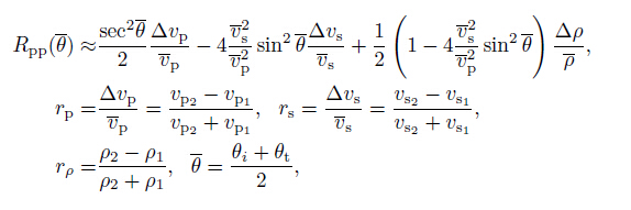
2 BACKGROUND THEORY 2.1 The Objective Function of InversionAki and Richards (1980) modified the result of Frasier and Richards and proposed the linearized P-wave reflectivity equation as
|
(1) |
where Rp, rs, rρ are reflection coefficients of P-wave velocity, S-wave velocity, and density, respectively. θ is the average angle of incidence and transmission angle. vp, vs are average P-wave velocity and S-wave velocity on the two sides of the interface, respectively. θ can be obtained by the a priori velocity model, and then equation
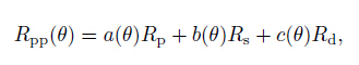
(1) can be written as follows
|
(2) |
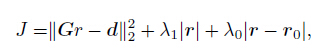
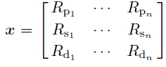
where Rp, Rs, Rd are reflection coefficients of P-wave velocity, S-wave velocity, and density, respectively. Eq.(2) is utilized for the forward modeling at any incidence on the interfaces. Therefore, the inversion objective function is initially constructed as
|
(3) |
|
(4) |
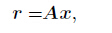
where r is the reflection coefficient. G is wavelet matrix and d is the observed seismic data.
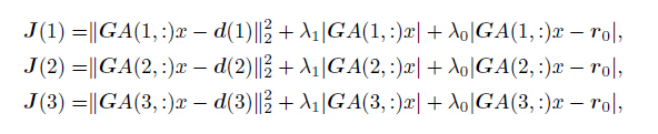
|
(5) |
where d (i), i = 1, 2, 3, … is the observed seismic data corresponding to different incidences, respectively. Inver- sion process is equal to minJ J T, where J = [J1 J2 J3].
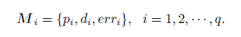
2.2 Inverse Operator Estimation AlgorithmThe inverse operator estimation algorithm (Růžek et al., 2009) works with q models, and each model M consists of three parts: parameter vector, data vector, and model error.
|
(6) |
The parameter vector can be regarded as objective elastic parameters, data vector is the synthetic seismogram and model error is the error between observed and synthetic data. The algorithm mainly contains the following four steps: initialization, selection, prediction, and correction. Basic information should be defined in the initialization part, such as the number of the objective parameters. In the selection part, suitable models can be generated which will be used for prediction. Then a solution can be obtained with prediction. At last some corrections should be made because of the difference between prediction methods and real case.
(1) Initialization
At this stage, all the necessary parameters should be defined and limited to reasonable ranges.
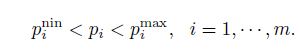
|
Initial model population is distributed randomly at a uniform probability in the allowed space. Models are sorted by error and the model with minimum error is considered as the best model so far.

|
(7) |
After each cycle, models should be arranged according to the following rules. The best model is set as the center and the others are surrounding it on the spherical surface at a uniform probability. R is the radius of the sphere or hypersphere.
(2) Selection
In the first cycle, R = 1. Suppose that {pc, R} is known, and then the new models will be generated by the following rules.
1) The best model {pc, dc, errc} is set as the first model.
2) Tensor Cm is written as Cm = LLT by Choleski decomposition.
3) Suitable model is estimated by pg = pc + RLg, where g is a random unit vector.
q models will be selected according to the error. In order to improve computational efficiency, the new model which is close to the existing model will be abandoned, and thus the number of forward modeling decreases.
(3) Prediction
q suitable models will be utilized for prediction of the candidate solutions. Population of prediction models→prediction algorithm→candidate solution Three different prediction algorithms are applied in this paper: linear regression, RBFN, and ‘Kriging’. These three algorithms are used cyclically, which is helpful to enhance the adaptability for an unknown inversion problem.
(4) Correction
The number of prediction model, the size of the population and the position of the center are important, which could be changed after each cycle. The number of prediction model influence the computation cost, but it affects the accuracy of the solution little. A proper q will be 3∼5 times of the number of objective parameters.The key is the position of the center and the size, which influences the results directly. As a result, the proper correction rules are made in each iteration. The number of consecutive iterations during which no improvement is reached is also monitored (nwait).
3 SYNTHETIC EXAMPLESA suite of well data containing P-wave and S-wave velocities and density well logging curves is utilized for the synthetic examples. The synthetic seismogram is generated by convolving Eq.(1) with a Ricker wavelet with the dominant frequency of 35 Hz. Then Eq.(5) is utilized to get the objective parameters. The inversion result is colored in blue in Fig. 2 when the synthetic seismic data is noise free, and the model value is colored in red and the initial value is colored in green. It is evident that inversion results are reasonable because there is little disparity between the red and blue curves in the case that the initial value is set as the result of the repeatedly smoothed model value.

|
Fig. 2 Inversion results of three parameters |
The random noise whose SNR is 3 is added to synthetic seismic data for noise immunity test. Fig. 3 shows the synthetic seismic data and Fig. 4 shows the inversion results. Overall, the inversion results keep a good consistency with model value, and inversion for density is unstable because it is a bottleneck of three-term AVO inversion.

|
Fig. 3 The comparison of synthetic seismogram (S/N=3) |

|
Fig. 4 Inversion results of three parameters when SNR is 3 |
Figure 5 shows the synthetic seismic data and Fig. 6 shows the inversion results when the S/N ratio is 1. It is feasible to estimate the three elastic parameters with moderate noise. Inversion values have a high correlation with the model values even if an opposite initial model is given. However, the inversion depends on the initial model more as the noise increases. In addition to looking for a better initial model, we can also control the number of cycles and threshold value to improve the accuracy of the inversion.

|
Fig. 5 The comparison of synthetic seismogram (S/N=1) |

|
Fig. 6 nversion results of three parameters when SNR is 1 |
This paper uses a non-optimal method, so the effect of L1 norm constraints and initial model need to be discussed from two aspects: stability and number of singular values.
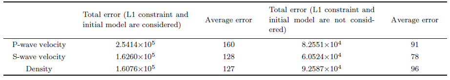
For the effect on stability, the inversion without L1 constraint and initial model was executed 10 times individually and the total error (Table 2) between the inversion value and model value can be obtained for both approaches respectively, as well as the average error. Then the average error is normalized at each sampling point (Fig. 7). Fig. 7 shows the relative magnitude of the error, and the absolute value is shown in Table 2. As a result, we can find that the error is smaller if L1 constraint and initial model are added in the inversion. In Fig. 7, the red curve represents the error without the constraint and the blue curve represents the error with them. We can notice that the range of red curve is from 0.3 to 1 for P-wave velocity and density, while the range of blue one maintained at 0.5, which indicates that L1 constraint and initial model help to stabilize the inversion.
|
|
Table 2 The total error and average error of the inversion results |

|
Fig. 7 Stability analysis with and without constraint and initial model |
Singular values result in redundant loop. As a result, the inversion without constraint is time consuming because the number of singular values is large. And the probability that singular value happens is 12/300. But if the constraint is added, the probability changes to 3/300. Overall, L1 constraint and initial model are feasible and effective in enhancing the stability and accuracy of inversion.
Lateral continuity is another key point in AVO inversion. A two-dimension model is utilized for lateral continuity test. Fig. 8 shows the synthetic seismic profiles with three different incident angles and the inversion results. The inversion results maintain a good lateral continuity.

|
Fig. 8 Synthetic seismograms and P-wave velocity, shear velocity, density inversion results |
Field data from a land area of China is utilized to test the feasibility of proposed inversion approach. Before AVO inversion, seismic data requires amplitude preservation processing including the spreading compensation, calibration of source and detector combination effects, inverse Q filtering, surface consistent processing, pre- stack denoising, removal of multiple waves and assuming multiples and anisotropy of interlayer are negligible. Fig. 9 shows the three partial angle stacked seismic profiles with different incident angles. The vertical axis represents time, and the horizontal axis is CDP and sample interval is 2 ms. Initial models are estimated from well information and a priori geological information. A better initial model helps to improve the inversion efficiency. The initial models and the inversion results are displayed in Fig. 10. Correlation between the initial models and inversion result is not very high, but reasonable results can still be obtained.

|
Fig. 9 The seismic profiles with 3 center incidences |

|
Fig. 10 The initial models and the inversion result |
As seen from Fig. 10, where the red part represents high value, the inversion results are reasonable (Fig. 9). The inversion results are consistent with the seismic profiles on energy response. Another inversion result is given by a commercial software, and the 70th trace from inversion resutls of the proposed approach and software are displayed together in Fig. 11, which verifies the credibility of the proposed inversion approach.

|
Fig. 11 70th trace from inversion of the approach proposed (red) and software (blue) |
In this paper, an inverse operator estimation algorithm is proposed for AVO inversion. The inversion objective function takes advantage of both Aki-Richards approximation equation and L1 constraint. Synthetic examples show that the new algorithm owns a high stability and accuracy which can be improved by adding constraints. Field data examples also produced reasonable results. The lateral continuity can be enhanced with initial model constraint. Overall, the proposed inversion algorithm shows great potential in AVO inversion.
ACKNOWLEDGMENTSWe would like to acknowledge the sponsorship of National Nature Science Foundation Project (U1562215), National Grand Project for Science and Technology (2016ZX05024-004), Natural Science Foundation of Shan- dong (BS2014NJ005), Science Foundation from SINOPEC Key Laboratory of Geophysics (33550006-15-FW2099- 0027) and the Fundamental Research Funds for the Central Universities.
| [1] | Aki K, Richards P G. 1980. Quantitative Seismology:Theory and Methods. USA:W H Freeman&Co. |
| [2] | Bortfeld R. 1961. Approximations to the reflection and transmission coefficients of plane longitudinal and transverse WAVES[J]. Geophysical Prospecting, 9 (4): 485–502. |
| [3] | Chen J J, Yin X Y. 2007. Three-parameter AVO waveform inversion based on Bayesian theorem[J]. Chinese J. Geophys., 50 (4): 1251–1260. |
| [4] | Downton J E, Lines L R. 2001. Constrained three parameter AVO inversion and uncertainty analysis.//CSEG 2001 expanded abstracts. 251-254. |
| [5] | Downton J E, Lines L R. 2004. Three term AVO waveform inversion.//SEG Technical Program Expanded Abstracts. 23(1):215-218. |
| [6] | Goodway W, Chen T, Downton J. 1997. Improved AVO fluid detection and lithology discrimination using Lam Petrophysical parameters "λρ μρ λμ fluid stack" from P and S inversions.//SEG Annual Meeting Expanded Abstracts. |
| [7] | Gray D, Andersen E. 2001. The application of AVO and inversion to the estimation of rock properties.//SEG Annual Meeting Expanded Abstracts. 70:549-552. |
| [8] | Kuzma H A, Rector J W. 2004. Non-linear AVO inversion using support vector machines.//74th SEG Annual Meeting Expanded Abstracts. |
| [9] | Ma X Q. 2001. Technical article:Global joint inversion for the estimation of acoustic and shear impedances from AVO derived P-and S-wave reflectivity data[J]. First Break, 19 (10): 557–566. |
| [10] | Mogensen S, Link C. 2001. Artificial neural network solutions to AVO inversion problems.//2001 SEG Annual Meeting Expanded Abstracts. |
| [11] | Press F. 1968. Earth models obtained by Monte Carlo inversion[J]. Journal of Geophysical Research, 73 (16): 5223–5234. |
| [12] | Růžek B, Kolář P, Kvasnička M. 2009. Robust solver of a system of nonlinear equations[J]. Technical Computing Prague. Shuey R T. 1985. A simplification of the Zoeppritz equations. Geophysics, 50 (4): 609–614. |
| [13] | Simmons J L Jr, Backus M M. 1996. Waveform-based AVO inversion and AVO prediction-error[J]. Geophysics, 61 (6): 1575–1588. |
| [14] | Tikhonov A N. 1963. Solution of incorrectly formulated problems and the regularization method[J]. Soviet Mathematical Doklady, 4 : 1035–1038. |
| [15] | Yin X Y, Zhang S X. 2014. Bayesian inversion for effective pore-fluid bulk modulus based on fluid-matrix decoupled amplitude variation with offset approximation[J]. Geophysics, 79 (5): R221–R232. |
| [16] | Yan P F, Zhang C S. 2005. Artificial Neural Networks and Evolutionary Computing [M]. Beijing: Tsinghua University Press . |
| [17] | Yang P J, Yin X Y. 2008. Non-linear quadratic programming bayesian prestack inversion[J]. Chinese J. Geophys. , 51 (6): 1876–1882. |
| [18] | Yin X Y, Wu G C, Zhang H Z. 1994. The application of neural networks in the reservior prediction[J]. Journal of the University of Petroleum , 18 (5): 20–26. |
| [19] | Yin X Y, Zhang S X, Zhang F C, Hao Q Y. 2010. Elastic impedance inversion for reservoir description and fluid identification based on Russell approximation[J]. Oil Geophysical Prospecting , 45 (3): 373–380. |
| [20] | Yin X Y, Zong Z Y, Wu G C. 2013. Improving seismic interpretation:a high-contrast approximation to the reflection coefficient of a plane longitudinal wave[J]. Petroleum Science, 10 (4): 466–476. |
| [21] | Yin X Y, Cao D P, Wang B L, Zong Z Y. 2014. Progress on fluid identification method based on pre-stack seismic inversion[J]. Oil Geophysical Prospecting , 49 (1): 22–34. |
| [22] | Yin X Y, Cui W, Zong Z Y, et al. 2014. Petrophysical property inversion of reservoirs based on elastic impedance[J]. Chinese J. Geophys. , 57 (12): 4132–4140. |
| [23] | Yin X Y, Zong Z Y, Wu G C. 2015. Research on seismic fluid identification driven by rock physics[J]. Science China Earth Sciences, 58 (2): 159–171. |
| [24] | Zheng X D. 1991. The approximate equations of Zoeppritz equation and its applications[J]. Oil Geophysical Prospecting , 26 (2): 129–144. |
| [25] | Zong Z Y, Yin X Y, Zhang F, et al. 2012. Reflection coefficient equation and pre-stack seismic inversion with Young's modulus and Poisson ratio[J]. Chinese J. Geophys. , 55 (11): 3786–3794. DOI: 10.6038/j.issn.001-5733.2012.11.025 |
| [26] | Zong Z Y, Yin X Y, Wu G C. 2012. AVO inversion and poroelasticity with P-and S-wave moduli[J]. Geophysics, 77 (6): N17–N24. |
| [27] | Zong Z Y, Yin X Y, Wu G C. 2013a. Elastic impedance parameterization and inversion with Young's modulus and Poisson's ratio[J]. Geophysics, 78 (6): N35–N42. |
| [28] | Zong Z Y, Yin X Y, Wu G C. 2013b. Multi-parameter nonlinear inversion with exact reflection coefficient equation[J]. Journal of Applied Geophysics, 98 : 21–32. |
| [29] | Zong Z Y, Yin X Y, Wu G C, et al. 2015. Elastic inverse scattering for fluid variation with time-lapse seismic data[J]. Geophysics, 80 (2): WA61–WA67. |