 2016, Vol. 59


Seismic exploration has advanced from the simple structure identification to the research of complex structures. From the existing data, such as seismic data, to obtain the high-resolution fluid indicator can be more effective for the reservoir prediction and fluid identification. Stochastic inversion is a kind of highresolution inversion method which is different from the conventional ones. Many scholars have carried out research on deterministic inversion and stochastic inversion (Francis et al., 2005, 2006; Moyen et al., 2009; Sams et al., 2008; Sancevero et al., 2005). Studies have shown that deterministic inversion gives only local smoothing estimation, and stochastic inversion method can provide a plurality of inversion results. Meanwhile it meets the actual seismic data and well-logging data. It also can reasonably estimate and reflect the uncertainty information that is smoothed out by deterministic inversion. Compared with stochastic inversion, the deterministic inversion method has the characteristics of good lateral continuity and fast calculation speed, so it has a wide application. Because of the slow calculation speed and other reasons (Dubrule, 1996), the use scope of stochastic inversion is relatively small. But in recent years the stochastic inversion can simulate the information out of seismic frequency band under the constraints of spatial correlation and well-logging data. Consequently, its resolution is higher than that of conventional deterministic inversion and stochastic inversion is becoming more and more attractive in recent years.
Many scholars in China and abroad proposed different types of fluid factors based on the elastic parameters. The earliest fluid factor is proposed by Smith et al.(1987), and it is a parameter composed of the weight calculation of the relative variation of longitudinal and transverse wave velocities. Goodway et al.(1997) proposed the LMR (Lamda-Miu-Rho) method using the Lame modulus to identify fluid. Biot (1941) and Gassmann (1951) studied the fluid factor construction method of porous fluid saturated rock respectively. Russell (2003) summarized the previous view and proposed the Russell fluid factor based on the theory of porous elastic medium. Quakenbush et al.(2006) applied the concept of Poisson impedance based on the Pimpedance and S-impedance. In order to reduce the accumulative error and the uncertainty in the calculation process, the scholars have made a lot of efforts to realize the reliable estimation of fluid factor. Wang et al.(2005) applied the elastic impedance inversion and parameter extraction method to the practical data and obtained good results. Subsequently, Wang et al.(2007) also derived elastic impedance equation including the Lame modulus based on Gray approximation, and realized the direct extraction of Lame parameters based on elastic impedance. Yin et al.(2010) derived the elastic impedance formula including Gassmann fluid items and studied the direct extraction method of Gassmann fluid items. Zong et al.(2011, 2012) explored the application of elastic impedance inversion in the fluid identification of carbonate and clasolite reservoirs. Zong et al.(2013) studied the direct extraction method of fluid factors in heterogeneous reservoirs. Yin et al.(2014) discussed the research progress of fluid identification method based on pre-stack seismic inversion, and presented a new fluid factor classification method.
The direct estimation method for the Russell fluid factor based on stochastic seismic inversion proposed by us provides sensitive and reliable data support for reservoir fluid identification. Here, we define the a priori information and likelihood function as Gaussian probability density. As a consequence of nonlinearity, no closed form expression of the posteriori probability density can be formulated. Therefore, we apply the Metropolis algorithm to obtain an exhaustive description of the posteriori probability density. Therefore, the inversion method based on Monte Carlo theory proposed in this paper combines the sequential Gaussian simulation and the Metropolis algorithm. Through the model data and real data analysis, it can be found that the direct estimation method for the Russell fluid factor is effective.
2 METHODSIn this paper, we use Bayesian theory to find the solutions of inversion problem. One of the advantages of applying Bayesian theory is that we can get uncertainty estimates when inverting fluid factor. Here, we get the Gaussian a priori probability density of Russell fluid factor through SGS. After that, we define the a priori information and likelihood function as Gaussian distribution and apply Metropolis algorithm to obtain an exhaustive description of the posteriori probability density of fluid factor. If the acceptance probability is satisfied, then the Russell fluid factor is obtained. If not, then the SGS is required. Fig. 1 is the flowchart of the direct estimation method for the Russell fluid factor based on stochastic seismic inversion.

|
Fig. 1 Flowchart of the direct estimation method for the Russell fluid factor based on stochastic seismic inversion |
Most fluid factors are based on single-phase medium theory, however, the rock-physics based on twophase medium theory is better for studying the effects of pore fluid on the elastic properties of rock medium. Russell fluid factor is the most commonly used two-phase fluid factor. In this paper, we study the direct estimation method for the fluid factor based on stochastic seismic inversion starting from the Russell fluid factor.
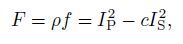
Russell et al.(2003) studied the relation between the elastic modulus and pore fluid of porous medium based on the Biot-Gassmann theory. They proposed Russell fluid factor in terms of the modified P-wave and S-wave velocity expressions (Well-logging data generally do not include shear wave velocity, which can be obtained by cross-dipole acoustic logging or full wave logging technology. In fact the shear wave velocity is calculated by porosity, clay content, water saturation and mineral modulus information through empirical relationships or equivalent theoretical model). The expression of Russell fluid factor can be represented as:
|
(1) |
where ρ means density of porous saturated fluid. IP is the P-wave impedance. IS is the S-wave impedance. c =(VP/VS)dry2 means the square of ratio of P-wave and S-wave velocity of dry rock. f characterizes the pore fluid effect, it is not only related to the fluid elastic effect, but also the integrated effect of rock solid parameters such as mineral matrix modulus, matrix modulus of dry rock, and the porosity. Therefore, Russell fluid factor has a high fluid sensitivity for the reservoir with mature consolidation and little change in porosity.
Many scholars have studied the computing method of parameter c. Russell (2003) proposed the computing method based on the laboratory measurement, but the cost of this method is relatively large. Yin (2010) proposed the computing method based on Gassmann equation. It estimates bulk modulus of the corresponding dry rock with rock physics theory, and then calculates the square of P-wave and S-wave velocity ratio of dry rock indirectly. In addition, we can apply empirical value as c = 2.233 or c = 2.333. We should determine the optimal parameter c according to the well-logging data of actual work area. In this paper, we apply the method of Yin (2010) based on the Gassmann formula.
2.2 Stochastic InversionIn this paper, we apply Russell fluid factor direct estimation method based on stochastic seismic inversion. It is a Monte Carlo based strategy for non-linear inversion, which is formulated in a Bayesian framework. According to the Bayesian theory:

|
(2) |
where ρ M (m) is a priori information of Russell fluid factor. L(d/m) is likelihood function, indicating the degree of match between observed and calculated synthetic seismic data. σ M (m) is the Bayesian posterior distribution. k is the normalized constant.
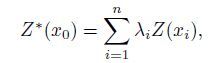
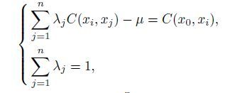
2.2.1 Geostatistical a priori informationThe sequential Gauss simulation (SGS) method is used to establish the geostatistical a prior information. The idea of sequential simulation is sequentially obtaining the conditional cumulative distribution function (CCDF) of every grid along the random simulation path, then getting the simulation value from the CCDF. SGS provides a most straightforward algorithm for the generation of a multivariable Gaussian field and it is made from one pixel to another sequentially. SGS is useful for the Gaussian field model, so the initial data must be Gaussian transformed. Thus the CCDF is Gaussian distribution, whose mean and variance can be got from the Kriging equations. Kriging linear estimator can be obtained by the linear weighted average value of the known regional variables as Eq.(3). In order to obtain the Kriging estimate, it needs to meet two conditions-linear unbiased estimation (Eq.(4)) and minimum variance (Eq.(5)), which can be expressed as:
|
(3) |
|
(4) |

|
(5) |
where Z (xi) is the known value. Z*(x0) is the value to be simulated. λi is the weighting coefficients of different known points. x0 is the point of simulation; μ is the Lagrange constant. δE2 is the posterior standard deviation. We can get the Kriging estimation value by minimizing the variance δE2 . C (, ) is the covariance function, which can be calculated by Eq.(6):

|
(6) |
where C (x0, xi) is the covariance of the known point and the estimated point. C (xi, xj) is the covariance of the two estimated points. N(h) is the total number of sample points whose separation distance is h. m is the mean of the samples, 
The previous sequential Gaussian simulation method adopts the way of simulating the whole trace or multiple simulation way to match the seismic data. In this paper, we use the sequential Gaussian simulation (SGS) in a new implementation way proposed by Zou et al.(2013) to construct the geostatistical a priori information. It simulates only one point and one grid rather than the whole trace at one time until all the grid nodes are simulated. When the simulated result is better than the initial model, we accept it and renew the initial model. Otherwise, the initial is kept. When the simulations of all the grids are finished, one realization is realized. After that the realization is repeated until meeting the convergence conditions. The simulation method not only can improve the computational accuracy of inversion results, but also can improve the computational efficiency.
2.2.2 Likelihood function constructionThe likelihood function using the following form:

|
(7) |
where di represents the amplitude of the simulated seismic waveforms. d obsi is the sample points of the observed data. σ is the standard deviation of expected data uncertainty. mi represents the inverted Russell fluid factor. m 0i is the low-frequency constraints used in the deterministic inversion (smooth constraints and point constraints). Therefore it overcomes the frequency missing problem caused by band-limited properties of the wavelet. When calculating synthetic seismogram we use the exact Zoeppritz equation, which can reduce the errors caused by Zoeppritz equation approximations.
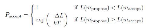
2.2.3 Metropolis algorithmMetropolis algorithm is a sampling method based on Monte Carlo theory (Mosegaard et al., 1995). Here, we define the a priori information and likelihood function as Gaussian probability density. As a consequence of nonlinearity, no closed form expression of the posteriori probability density can be formulated. Therefore, we apply the Metropolis algorithm to obtain an exhaustive description of the posteriori probability density. The Metropolis rule can be represented as:
|
(8) |
where L is likelihood function. maccept is the previously accepted model. mpropose is a sample from the a priori probability density, which is the perturbation of maccept. ΔL = L(mpropose)- L(maccept), k and T is adjustable parameters. Paccept is the probability of acceptance. Tarantola (2005) mentioned in his book that the acceptance probability of Metropolis rule should be kept between 30%~50%. If the acceptance probability is too high, the search speed in model space is slow. If the acceptance probability is too low, it will waste more computer resources to test the model that is not accepted. So we should adjust the variable parameters to keep the acceptance probability at about 30%~50%.
In summary, we obtain the geostatistical a priori information by the improved sequential Gaussian simulation method based on Bayesian theory framework. Construct the likelihood function using the low-frequency constraint information of deterministic inversion. Finally, apply the Metropolis algorithm to obtain the samples of posteriori probability density for fluid identification.
3 MODEL TEST AND ANALYSIS 3.1 Case Study with 1D Real DataHere we choose 1D real data to test the proposed estimation method and the data is the real well-logging data. Then calculate the synthetic seismic data by convolution model as pre-stack seismic data to invert for the fluid factor based on the existing well-logging data. Fig. 2 is the comparison of real data and estimation results, which are the inversion results of Russell fluid factor, Pwave velocity and density respectively. It can be seen from the figure that the inversion results are nearly in accordance with the real data. Figs. 3a and 3b are the comparison of real data and estimated fluid factors (Russell fluid factor, P-wave velocity and density) when the signal to noise ratio (S/N) is 4 and 1 respectively. We can see that even adding noise into the original data, the inversion results are still credible. Through the model test, it can be found that the inversion method has good robustness.

|
Fig. 2 Comparison of model and inversion results Black: all the inversion results; Red: mean of inversion results; Blue: model data (similarly hereinafter). |

|
Fig. 3 Comparison of model and inversion results (a) S/N=4; (b) S/N=1. |
We choose a part of Marmousi2 model to test and analyze the direct estimation method for the Russell fluid factor. Fig. 4 is a comparison of inversion result with model data. Fig. 4a is the model data, Fig. 4b is the extracted 12 pseudo wells, Fig. 4c is the estimated Russell fluid factor and Fig. 5 is the estimation result when S/N is 4. By comparing Figs. 4c and 4a, we can see that the estimation result is nearly in accordance with the model data, and it can identify thin layers. We can see that the resolution of fluid factor is relatively high. From the figure 5, we can see that even in the presence of noise, we can still obtain a reasonable inversion result. So Russell fluid factor based on the two-phase medium theory can represent the pore fluid effect on the rock medium and the estimation method we proposed is effective.

|
Fig. 4 Comparison of fluid factor inversion result with model data (a) Model data; (b) 12 pseudo wells; (c) Inversion result. |

|
Fig. 5 Comparison of fluid factor inversion result with model data when S/N=4 |
The real data is from an actual work area. The longitudinal sampling rate of seismic data is 2 ms, time range is from 1.122 s to 1.302 s, and we have a total of 101 traces of seismic data. Fig. 6 shows the post-stack seismic profile. Fig. 7 is the inverted Russell fluid factor. To test the feasibility of the proposed estimation method, we perform the blind well test (Well C is the blind well). It can be seen that the inversion result matches the well-logging data very well. Because the stochastic inversion method is used, the resolution is relatively high, which can be seen from the comparison of seismic data and inversion profile. The application of real data verifies the feasibility of the proposed inversion method.

|
Fig. 6 Poststack seismic profile (Black curve represents Russell fluid factor) |

|
Fig. 7 Inverted Russell fluid factor (Black curve represents Russell fluid factor) |
Russell fluid factor is a sensitive indicator for reservoir fluid indication. The direct estimation method for the Russell fluid factor based on stochastic seismic inversion is an efficient method for fluid identification, which is based on the Bayesian theory framework. In this paper we calculate the geostatistical a priori information of fluid factor through the improved sequential Gaussian simulation (SGS). Then construct the likelihood function based on the deterministic inversion. Finally, use Metropolis algorithm to sample the posteriori probability density and get the inversion results. From the data analysis, we can obtain effective fluid factor with the proposed fluid factor estimation method and it improves the precision of fluid indication.
ACKNOWLEDGMENTSThe work is sponsored by the National Basic Research Program of China (973 Program,2013CB228604),Major National Science and Technology Projects (2011ZX05009),the National Natural Science Foundation of China (41204085) and Natural Science Foundation of Shandong Province (ZR2011DQ013).
| [1] | Biot M A. 1941. General theory of three-dimensional consolidation[J]. Journal of Applied Physics, 12 (2): 155–164. |
| [2] | Dubrule O, Dromgoole P, Vankruijsdijk C. 1996. Workshop report:'Uncertainty in reserve estimates' EAGE Conference, Amsterdam, 2 June 1996[J]. Petroleum Geoscience, 2 (4): 351–352. |
| [3] | |
| [4] | Francis A M. 2006a. Understanding stochastic inversion:Part 1[J]. First Break, 24 (11): 69–77. |
| [5] | Francis A M. 2006b. Understanding stochastic inversion:Part 2[J]. First Break, 24 (12): 79–84. |
| [6] | |
| [7] | Goodway B, Chen T, Downton J. 1997. Improved AVO fluid detection and lithology discrimination using Lam petrophysical parameters; "λρ", "µρ", & "λ/µ fluid stack", from P and S inversions.//Proceedings of the 67th Annual International Meeting, SEG. Expanded Abstracts, 183-186. |
| [8] | Mosegaard K, Tarantola A. 1995. Monte Carlo sampling of solutions to inverse problems[J]. Journal of Geophysical Research, 100 (B7): 12431–12447. |
| [9] | Moyen R, Doyen P M. 2009. Reservoir connectivity uncertainty from stochastic seismic inversion.//Proceedings of the 79th Annual International Meeting, SEG. Expanded Abstracts, 2378-2382. |
| [10] | |
| [11] | Russell B H, Hedlin K, Hilterman F J, et al. 2003. Fluid-property discrimination with AVO:A Biot-Gassmann perspective[J]. Geophysics, 68 (1): 29–39. |
| [12] | Sams M, Saussus D. 2008. Comparison of uncertainty estimates from deterministic and geostatistical inversion.//Proceedings of the 78th Annual International Meeting, SEG. Expanded Abstracts, 1486-1490. |
| [13] | |
| [14] | Smith G C, Gidlow P M. 1987. Weighted stacking for rock property estimation and detection of gas[J]. Geophysical Prospecting, 35 (9): 993–1014. |
| [15] | Tarantola A. 2005. Inverse Problem Theory and Methods for Model Parameter Estimation[M]. Philadelphia: SIAM . |
| [16] | Wang B L, Yin X Y, Zhang F C. 2005. Elastic impedance inversion and its application[J]. Progress in Geophysics , 20 (1): 89–92. DOI: 10.3969/j.issn.1004-2903.2005.01.017 |
| [17] | Wang B L, Yin X Y, Zhang F C. 2007. Gray approximation-based elastic wave impedance equation and inversion[J]. Oil Geophysical Prospecting , 42 (4): 435–439. |
| [18] | |
| [19] | Yin X Y, Cao D P, Wang B L, et al. 2014. Research progress of fluid discrimination with pre-stack seismic inversion[J]. Oil Geophysical Prospecting , 49 (1): 22–34. |
| [20] | |
| [21] | |
| [22] | Zong Z Y, Yin X Y, Wu G C. 2012. Fluid identification method based on compressional and shear modulus direct inversion[J]. Chinese Journal of Geophysics , 55 (1): 284–292. DOI: 10.6038/j.issn.0001-5733.2012.01.028 |
| [23] | Zong Z Y, Yin X Y, Wu G C. 2013. Direct inversion for a fluid factor and its application in heterogeneous reservoirs[J]. Geophysical Prospecting, 61 (5): 998–1005. |
| [24] | Zou Y M, Zhou H, Guan S J, et al. 2013. A new implementation procedure of sequential Gaussian simulation in stochastic seismic inversion.//Proceedings of the 83th Annual International Meeting, SEG. Expanded Abstracts, 3113-3117. |