2 Acquisition Technique Supports, Bureau of Geophysical Prospecting, China National Petroleum Corporation, Zhuozhou Hebei 072751, China;
3 Institute of Geophysics and Planetary Physics, University of California at Santa Cruz, CA 95064, U. S. A.
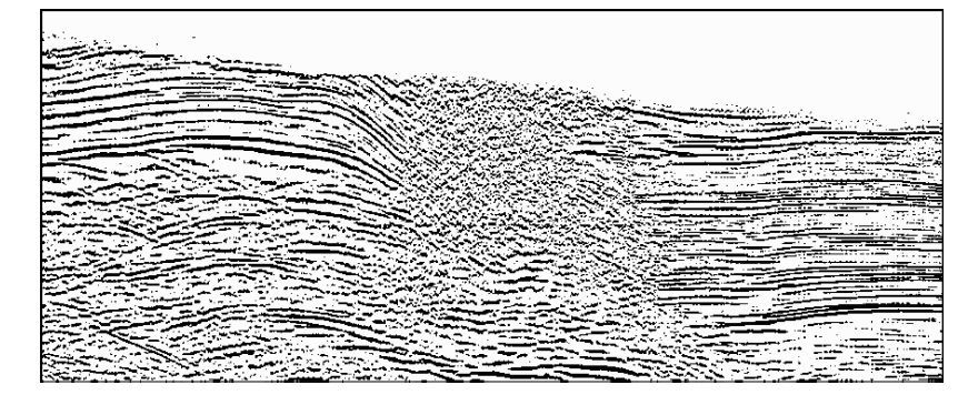
Reflection seismology is widely used for detecting the subsurface structures, and becomes an important technique for oil and gas exploration. High quality seismic image relies not only on high-quality seismic data and proper migration method, but also on accurate migration velocity model. Although significant progresses in data acquisition and migration method have been made, there remain unsolved problems in complex geological areas. In land acquisition, particularly inWestern China, the near surface layer is often dominated by small-scale heterogeneities from weathering, loose sediments or rugged topography, etc. Strong scatterings generated in this layer can seriously affect the quality of seismic data and the following depth imaging. As an example, shown in Fig. 1 is a seismic profile obtained inWestern China. On the left side of the profile is the mountain area and on the right side is the Gobi area. Satisfactory images can be obtained in both areas. However, the middle section of the profile corresponds to the piedmont zone composed of thick gravels, where the image is deteriorated due to the near surface small-scale heterogeneities. The small-scale heterogeneities affect the image from various aspects. Shallow scattering attenuates coherent energy from primary reflections. Meanwhile, the coda waves generated by multiple scattering add strong noise to the data. In addition, the small-scale structures often cannot be built into the migration model by conventional velocity building methods. The high-wavenumber errors in the model cause additional focusing problems in the imaging process. The above mentioned problems exist widely in land acquisition. During the data acquisition, affected by the mountainous areas, desert, piedmont zone, and very rugged terrains, the seismic data are highly complicated and characterized by very low signal-to-noise ratios and all types of interferences, making the subsequent data processing and explanation highly difficult (Xia et al., 2003). This problem attracted wide attention from both industrial and academic researchers. Various methods, e.g., 2D wide azimuth acquisition, wide line and geophone continuous array seismic acquisition, Macro-bin stack, etc., were proposed to solve this problem (Tang et al., 2014; Wu et al., 2012). The sole or joint application of these methods achieved certain results in areas with relatively simple geological structures (Ning et al., 2014). However, in the piedmont zone with very thick gravel beds or mountainous areas with complex topography, these methods have limited effect or even totally failed.
|
Fig. 1 Seismic image in a piedmont zone in Western China |
Although the problem itself and its serious effects are well known in the acquisition practice, and a number of field experiments have targeted to solve this problem, there is lack of an effective way to put this phenomenon under systematic investigation and an objective judgment to evaluate the proposed methods. The purpose of this paper is to integrate the related factors in the process (e.g., the shallow small-scale heterogeneities, the formation of the scattering noise, the attenuation of the signal and their effects on the fidelity of the image) with a unified numerical model, to quantify their effects on the depth image. We introduce the random velocity model to simulate the near surface velocity, thus a few statistical parameters can be used to characterize the highly complicated small-scale heterogeneities. In the meantime, we introduce the point spreading function (PSF) as the generalized image. The PSF and its amplitude and phase spectra in the wavenumber domain provide useful information to characterize the quality of the image. We then calculate PSFs numerically for given random velocity models, to create relations between the statistical parameters of random models and the properties of PSFs. In this way, we parameterize both the velocity model and the image quality, making it possible to form a concise relationship between the two, and the resulted method can be used to investigate how shallow heterogeneities can affect the depth image.
2 RANDOM VELOCITY MODEL AND POINT SPREADING FUNCTIONTo quantify the near-surface small-scale velocity perturbations and the quality of the depth image, we introduce random velocity model and point spreading function.
2.1 Random Velocity Models for Small-Scale HeterogeneitiesThe small-scale heterogeneities can be simulated with random media, and characterized by a few statistical parameters, in which the random spectral type (e.g., Gaussian, exponential or self-similar) gives the distribution of scatters of different sizes, the RMS perturbation gives the magnitude of the perturbation relative to the background velocity, and the correlation length gives the dominant scale of the heterogeneities. The interaction between the waves and the heterogeneities can be investigated by choosing right parameters to create random velocity model and using numerical simulations, which has been widely used in seismology (e.g., Frankel and Clayton, 1986; Xie and Lay, 1994; Wu et al., 2000; Xie et al., 2005a; Xie, 2013). Xi and Yao (2004a, 2004b), Ma et al.(2013) analyzed the wavefield characteristics in 2D elastic and viscoelastic random media, and applied them to some exploration problems. Xu et al.(2007), Liu et al.(2007a, 2007b) investigated kinetic and dynamic properties of seismic wave propagation in the random media. Han et al.(2015) investigated the wave front healing effect of wavefield in random media. Here, random velocity models with exponential type spectra are used to simulate the shallow small-scale heterogeneities for numerical experiments and related investigations.
2.2 Seismic Resolution and Point Spreading FunctionResolution analysis provides measures to evaluate the fidelity of seismic image reconstructed by the migration process. The PSF gives the resolution of the depth image and carries full information that affects the quality of the image. Gelius et al.(2002), Xie et al.(2005b, 2006), Wu et al.(2006) investigated the relationship between the PSF and seismic illumination in wavenumber domain. Xie et al.(2005b), Mao and Wu (2011), Valenciano et al.(2015) adopted the resolution information from PSF to improve the quality of the depth image. Cao (2013) proposed the method that directly calculates the PSF by imaging a single scattering point. Chen and Xie (2015) further discussed this method to avoid high order scatterings. High fidelity image relies on correct amplitude and phase in the wavefield. Therefore, the amplitude and phase in the PSF can be used as criteria in investigating the image quality. The resolution of image is affected by various factors such as the acquisition aperture, source frequency band, complexity of the overburden structure and the accuracy of the velocity model, etc. Therefore, the PSF and its amplitude and phase error can be used for investigating how those factors affect the image quality.
The seismic image obtained by migration is an approximate description of the actual subsurface structure. Namely, the image is a distorted version of the structure. The image at location can be described as the convolution between the PSF and velocity model (Xie et al., 2005b; Cao, 2013; Chen and Xie, 2015):

|
(1) |
where I(x) is the image, R(x) is the PSF, and m (x) is the velocity model perturbation, * denotes the spatial convolution. Ideally, R(x) can be a δ function and the image can reflect the actual structure. However, due to the illumination issue, R(x) is usually a complex distribution, which smears the image and causes its distortion. In the wavenumber domain, Eq.(1) becomes

|
(2) |
where k is the wavenumber, and I(k), R(k) and m (k) are transforms of I(x), R(x) and m (x) in the wavenumber domain. Replacing the velocity perturbation m (x) with a point scatterer, i.e., a δ function, we have

|
(3) |
In other words, the image of a point scatterer can be seen as the PSF for a given velocity model and acquisition system, and can be used to investigate the effects of the entire system (the acquisition system and overburden velocity) in the imaging process. We use this method to investigate the effect of near surface shallow heterogeneities on the image quality. The numerical method for calculating the response to a point scatterer can be either the embedded scattering point method (Cao, 2013, Chen and Xie, 2015) or the staining algorithm (Chen and Jia, 2014).
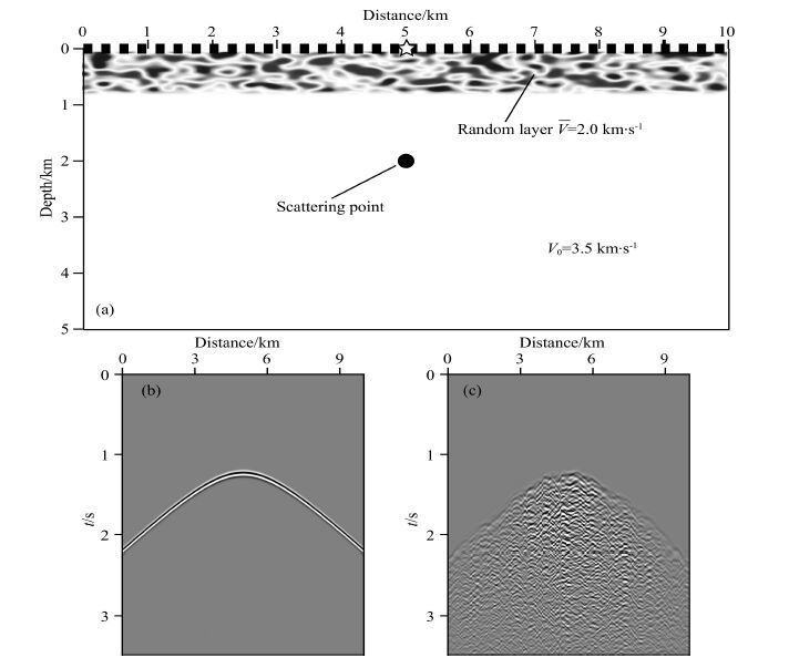
3 THE EFFECT OF SHALLOW SCATTERING ON SEISMIC DATA AND IMAGE RESOLUTION 3.1 The Effect of Shallow Scattering on SeismogramsTo test how a shallow random layer can affect the seismic data and the depth image, we use a two-layer velocity model shown in Fig. 2 to generate synthetic seismograms. The size of the model is 10 km×5 km, and the grid size is 10 m×10 m. The velocities in the top and bottom layers are 2.0 km·s-1 and 3.5 km·s-1, respectively. The exponential type random velocity perturbation is added to the top layer to simulate shallow heterogeneities. The layer thickness h, horizontal and vertical correlation lengths ax and az, and root mean square perturbation RMS are variables to simulate different near surface small-scale heterogeneities. To simplify the description, the velocity model with two homogenous layers is referred as background model, and the model with random perturbation top layer is referred as true model. A single scattering point is set at distance 5.0 km and depth 2.0 km as the target. A 15 Hz Ricker source is located on the surface at distance 5.0 km. Receivers are distributed on the entire surface.
|
Fig. 2 Cartoon showing the velocity model for numerical calculations |
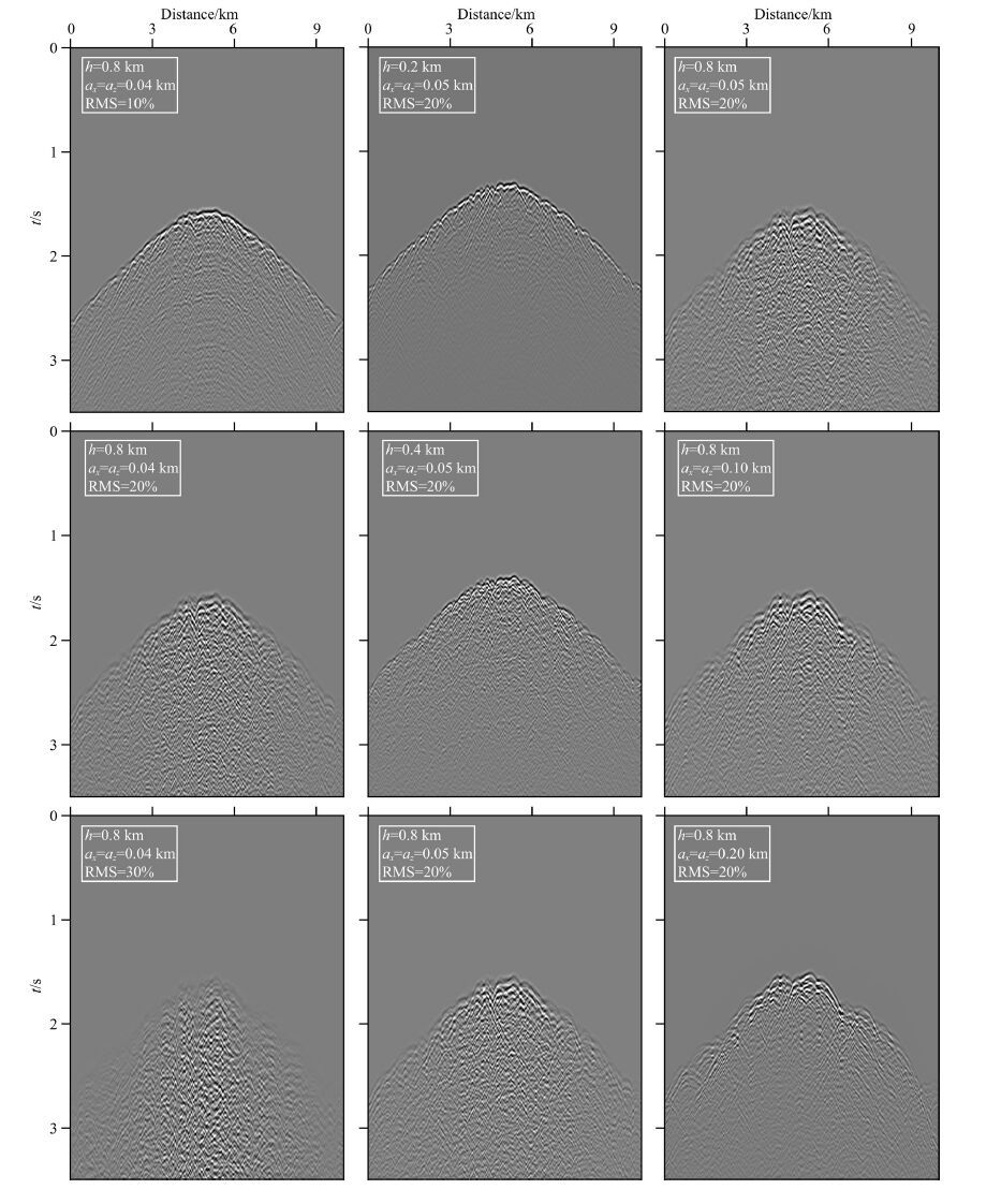
First we investigate the effect of shallow scattering on seismograms. The data recorded on the surface are waves scattered from the point scatterer and travel twice in the random layer. The record length is 3.5 s, and the sampling interval is 0.01 s. To illustrate the detailed characteristics, the direct wave is muted from the data. When there is no random layer, a parabolic event with definite arrival appears in the data as shown in Fig. 2b. In contrast, with the random layer in the model, the wave is scattered significantly when passing the layer twice. Hence, part of the energy is transferred from the primary arrival to the coda wave as shown in Fig. 2c. Random layers with different parameters, e.g., RMS perturbation, layer thickness and correlation length, are used to investigate their effects on the synthetics. Shown in Fig. 3 are shot gathers from the model with a random layer of various parameters. In the left column, the thickness of the top layer is fixed as h=0.8 km, the correlation lengths are ax = az = 40 m, and the root mean square velocity perturbations are RMS=10%, 20%, 30%. In the central column, ax = az = 50 m, RMS=20%, and h=0.2 km, 0.4 km, and 0.8 km. In the right column, h=0.8 km, RMS=20%, and ax = az = 50 m, 100 m, 200 m.
|
Fig. 3 Synthetic shot gathers from models with exponential random layers |
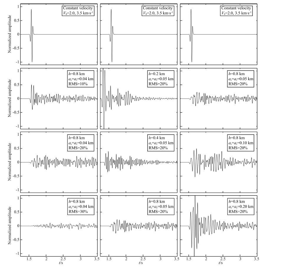
Shown in Fig. 4 are traces of synthetic seismograms recorded at 3.5 km on the surface. As references, listed in the top row are synthetics in the background model, where the velocity perturbation is zero. Other figures are corresponding to those in Fig. 3. For easy comparison, all traces are normalized with the amplitude in the background model. The seismogram in the background model is the single scattering from the point scatterer and appears as an impulse. On the contrary, in models with shallow random layer, part of the energy is transferred from the first arrival to the coda wave, due to multiple scatterings when waves passing through the random layer twice. With the increase of scatterings, e.g., by increasing the RMS perturbation (the left column) or layer thickness h(the central column), multiple scatterings gradually dominate the waveforms and turn the impulse into a wave train. In the right column, for fixed RMS perturbation and layer thickness h, changing the correlation length ax and az also strongly affects the result, which indicates that the scattering process is also controlled by the wavelength versus the scales of heterogeneities. The migration imaging is based on Born approximation. The loss of energy from the primary reflections and the development of the coda wave reduce the coherent information in the signal and generate noise in the image.
|
Fig. 4 Seismic waveforms from models with different shallow random layers |
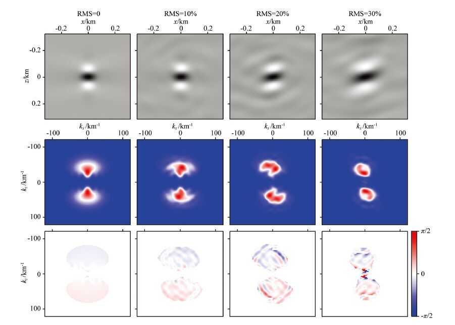
We use numerical method to investigate how the shallow random layer can cause errors in the amplitude and phase of a PSF. The same velocity model shown in Fig. 2 is used here. The sources are distributed on the entire surface with an interval of 0.5 km. We generate the synthetic data for given velocity models, and use the RTM to obtain the PSF by imaging the point scatterer. The thickness of the random layer is h=0.8 km and the correlation length ax = az = 40 m. First, we use the true velocity model to do the RTM, i.e., assuming all small-scale heterogeneities are exactly known. The results are shown in Fig. 5, where in the top row are PSFs calculated in models with RMS=0, 10%, 20%, and 30%, respectively. The second and third rows are their corresponding amplitude and phase spectra in wavenumber domain. The horizontal and the vertical axes are horizontal and vertical wavenumbers respectively. The first and second rows are normalized separately, and the phases are normalized to ±π/2. The results show that the image quality is seriously affected by the multiple scatterings in the random layer. However, the PSF can still focus at the right location if the small-scale heterogeneities are exactly known. From the amplitude spectra, we see that, with the increase of the scattering, the PSF loses coherent information gradually from high to low wavenumbers, but their phase errors are mostly within ±π/2, which is the premise for constructive interference.
|
Fig. 5 Spatial and wavenumber domain PSFs obtained using true velocity model |
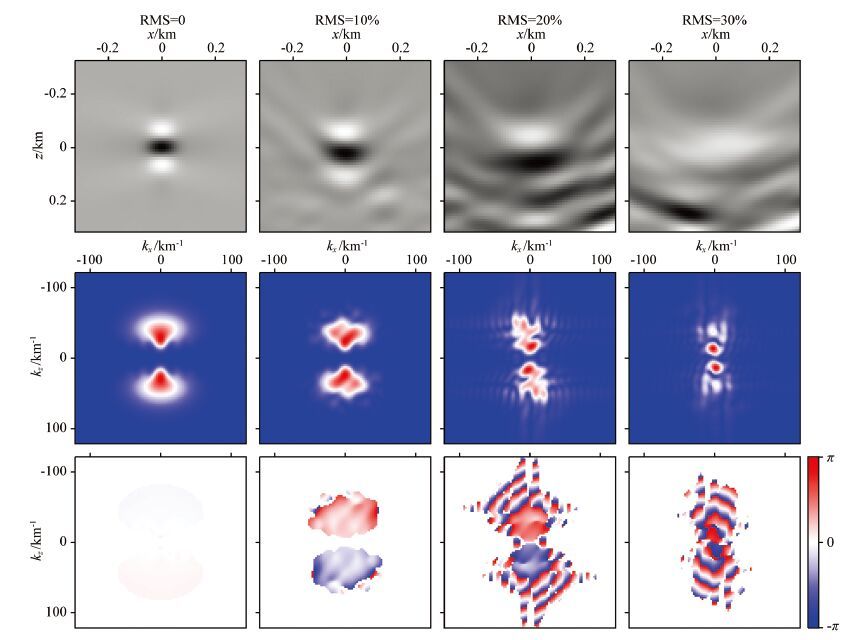
In practice, it is often impossible to build migration velocity model down to very small scale. Shown in Fig. 6 are PSFs calculated using the background model (assuming the small-scale heterogeneities are unknown and an average velocity is used instead). Comparing Figs. 5 and 6, we see that the PSF quickly loses focusing (row one) as the scattering increases. The amplitude spectra quickly lose their high wavenumber components. The most apparent changes are in phases. With the increase of velocity perturbations, the phases quickly go to random and lose coherence (note here the phases are normalized within ±π). With strong attenuation of amplitudes and random undulation of phases, the extrapolated wavefields cannot satisfy the stationary condition, thus fail to generate proper image.
|
Fig. 6 Space and wavenumber domain PSFs obtained using background velocity model |
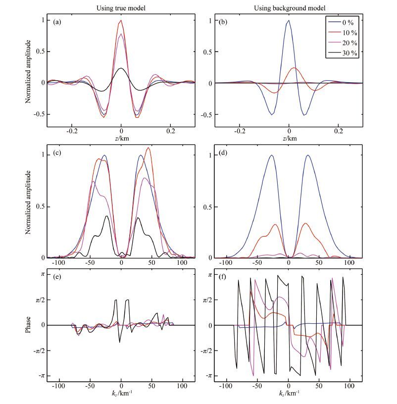
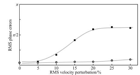
Figure 7 further compares the influence of the near-surface random layer to PSFs by comparing their vertical profiles under different velocity perturbations. Illustrated in the left column are results calculated in the true model, and in the right column are calculated in the background model. When the true velocity model is used, the increase of the velocity perturbation apparently reduces the amplitude of the PSF, but the result is still unbiased. However, if the small-scale heterogeneities are unknown, not only are the amplitudes strongly affected, but also the PSFs cannot focus at their right location. With RMS=20%, the amplitude spectrum almost approaches to zero, and the phases are essentially random due to phase wrapping. Actually, these results are obtained without noises other than the shallow scatterings. Considering the noise from other sources, the image is practically impossible. The mean value of the phase errors in Fig. 5 and Fig. 6 should be zero. Thus to quantify the influence of the small-scale heterogeneities, the RMS phase errors biased from zero are used and shown in Fig. 8. The result reveals that, although increasing with the perturbation, the RMS phase errors are comparatively small when true model is used. However, when the small-scale heterogeneities are unknown, the RMS phase errors increase much more quickly. Zero-phase condition is the basis for seismic imaging. When phase errors are less than 1/4 cycle (π/2), the constructive interference makes individual frequency components be superposed and contribute to the final image. Otherwise, the destructive interference will cause the difficulty in imaging. From the results in Fig. 8, with the background model and acquisition system in Fig. 2, when the RMS velocity perturbation is 5%, the phase error is relatively small. When the velocity perturbation increases to 10%~15%, the phase error increases quickly. Due to phase wrapping, measured phases are limited to ±π. When the velocity perturbation is over 20%, the RMS phase error reaches a saturated value. Note that the velocity error primarily causes the travel time error. Given the travel time error, the phase spectra of highfrequency component will be affected more severely. From the amplitude and phase spectra in Fig. 6, the influences of the small-scale heterogeneities deteriorate the spectra from high wavenumber components to the low wavenumber components as the perturbation increases. Hence, the velocity error from small-scale heterogeneities will first affect the imaging of small-scale structures. As the error increases, the images of the large-scale structures are gradually affected. In other words, low-frequency signals have better performance in resisting the small-scale scattering. Therefore, in strongly scattered area, properly extending the source towards the lower frequency is at least beneficial to the imaging of large-scale structures.
|
Fig. 7 Influence of the near-surface random layer on PSFs |
|
Fig. 8 Influence of a shallow random velocity layer to the phase error of a subsurface PSF |
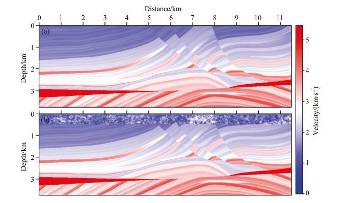
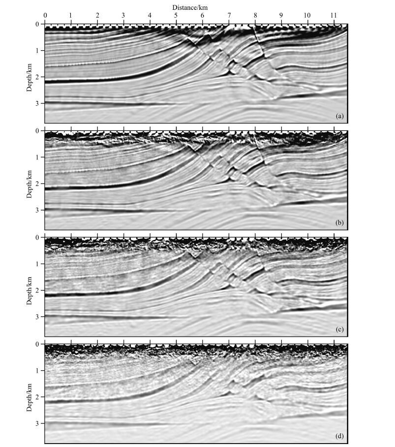
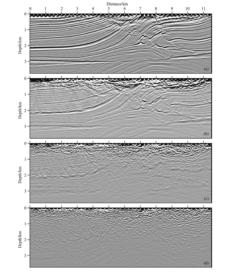
To test how the random layer will affect the depth image, we modify the original Marmousi model (Bourgeois et al., 1991) for numerical experiments. Shown in Fig. 9a is the original model, and in Fig. 9b is the modified version, where the top 0.5 km is overlapped by a random layer with correlation length ax = az = 40 m and variable RMS velocity perturbations. The source is a 15 Hz Ricker wavelet. Illustrated in Fig. 10 are depth images calculated in the true velocity models, assuming all small-scale heterogeneities are exactly known. As a comparison, Fig. 10a is the conventional depth image, where both the forward modeling and migration imaging are calculated using the original Marmousi model. Figs. 10b-10d are results calculated using the modified model with shallow perturbations of RMS=10%, 20%, and 30%. In the calculation, both the synthetic data and the depth image are calculated using the model with perturbations. Although the image quality is affected by the small-scale heterogeneities, and the influence increases as the perturbation becoming stronger, the results show that the subsurface image can still be obtained if the exact velocity models with small-scale heterogeneities are used in the migration. Shown in Fig. 11 are imaging results assuming the small-scale heterogeneities are unknown. Fig. 11a is the conventional depth image for comparison. In Figs. 11b-11d, the synthetic data are generated using the modified models with shallow RMS velocity perturbations of 10%, 20%, and 30%. However, the migration imaging is calculated in the original model. The results show that when the RMS is 10%, certain major structures can be narrowly seen in the image. However, when the RMS reaches 20%~30%, it is almost impossible to obtain the image. Consequently, if small-scale heterogeneities are unknown and the background model is used in the migration, the image can be seriously affected or even completely missed. This is consistent with the phenomenon seen in Western China as shown in Fig. 1 and supported by the analysis shown in Fig. 8.
|
Fig. 9 Modified Marmousi model |
|
Fig. 10 Prestack depth images obtained using true velocity models (assuming the small-scale fluctuations are known) |
|
Fig. 11 Prestack depth images obtained using original Marmousi model without the top random layer (assuming the small-scale fluctuations are unknown) |
Strong near surface scatterings in land acquisition can cause difficulties in seismic data acquisition and depth imaging. The influence lies in two aspects: First, the energy of seismic wave is strongly attenuated and scattered by the near surface small-scale heterogeneities, thus the signal-to-noise ratio is reduced. Second, the lack of small-scale heterogeneities in velocity model will cause travel time or phase errors, making focusing difficulty in the image. The small-scale heterogeneities can be characterized by the random media, which can be used for investigating their influence on wave propagation, scattering and imaging. The point spreading function and its amplitude and phase spectra carry the information regarding the fidelity of the imaging process, providing a measure of the image quality. By combining the above two together, we propose a method to analyze how the small-scale heterogeneities in the near surface layer can affect the seismic data and the quality of seismic migration.
Numerical calculations are used to create relations between the statistical parameters of the random model and the characteristics of the resolution. Numerical experiments show that the quality of the data acquisition and depth image are affected by the thickness, RMS velocity fluctuation and correlation length of the smallscale heterogeneities in the near surface random layer. The image quality deteriorates when either the velocity perturbation or the thickness of the random layer increases. The influence of the correlation length of the smallscale heterogeneities is highly complicated. In general, the scattering effect dominates when ka = 1. However, it needs further study in the case of broadband imaging. The results reveal that the near surface random layer will affect the accuracy of the depth image. When the small-scale heterogeneities in the near surface random layer are known, the image quality can be improved; On the contrary, when the small-scale heterogeneities are totally unknown, proper focusing becomes very difficult or even impossible. It implies that compensating the intermediate- to small-scale variations in velocity building (e.g., the joint implementation of shallow velocity inversion, wave equation datuming and topographic correction) may significantly improve the image quality. Besides, the high-frequency content in seismic signal is affected more seriously than the low-frequency part, thus boosting the low-frequency content of the source would also improve the image quality. The primary purpose of this research is developing an analytical tool, which links major factors in the small-scale velocity model to the quality of the depth image. Under this framework, various methods proposed for solving this problem can be systematically tested and reviewed.
5 CONCLUSIONIn land acquisition, strong scatterings generated by the near surface layer dominated by small-scale heterogeneities can seriously affect the quality of data acquisition and depth image. In this paper, we introduce the random velocity model to simulate the near surface velocity, thus a few statistical parameters can be used to characterize the highly complicated small-scale heterogeneities. In the meantime, we introduce the point spreading function (PSF) as the generalized image. The PSF and its amplitude and phase spectra in wavenumber domain provide useful information to characterize the quality of the image. We then calculate PSFs numerically for given random velocity models to create relations between statistical parameters of random models and the properties of PSFs. In this way, we parameterize both the velocity model and the image quality, making it possible to create a concise relationship between the two. The resulted method can be used to investigate how shallow heterogeneities can affect the depth image, and it is promising to be used in judging the existing methods targeted to overcome the effect of the near surface scattering and the new methods currently under developing. In the future work, more complicated cases where parameters change with the depth, elastic random media and the influence of irregular free-surface should be considered.
ACKNOWLEDGMENTSThis research is supported by the WTOPI Research Consortium at the University of California, Santa Cruz.
| [1] | Bourgeois A, Bourget M, Lailly P, et al. 1991. Marmousi, model and data.//The Marmousi Experience:5-16. |
| [2] | Cao J. 2013. Resolution/illumination analysis and imaging compensation in 3D dip-azimuth domain.//83rd Annual International Meeting, SEG, Expanded Abstracts, 3931-3936. |
| [3] | Chen B, Jia X F. 2014. Staining algorithm for seismic modeling and migration[J]. Geophysics, 79 (4): S121–S129. |
| [4] | Chen B, Xie X B. 2015. An efficient method for broadband seismic illumination and resolution analyses.//85th Annual International Meeting, SEG, Expanded Abstracts, 4227-4231. |
| [5] | Frankel A, Clayton R W. 1986. Finite difference simulations of seismic scattering:implications for the propagation of short-period seismic waves in the crust and models of crustal heterogeneity[J]. Journal of Geophysical Research, 91 (B6): 6465–6489. |
| [6] | Han Y Y, Zhang Z J, Liang K, et al. 2015. Seismic wave field modeling of wave front healing effect in self-organized media using a heterogeneous multi-scale method[J]. Chinese J. Geophys., 58 (2): 643–655. DOI: 10.6038/cjg20150225 |
| [7] | He Y, Xie X B, Lay T. 2008. Explosion-source energy partitioning and Lg-wave excitation:contributions of free-surface scattering[J]. Bull. Seism. Soc. Am., 98 (2): 778–792. |
| [8] | Liu Y X, Xu C M, Ning J R. 2007a. Comparison of acoustic propagation in several different types self-organized media[J]. Chinese J. Geophys., 50 (3): 830–836. |
| [9] | Liu Y X, Xu T, Zhao B, et al. 2007b. Seismic sounding of anisotropic self-similar self-organized medium[J]. Chinese J. Geophys., 50 (1): 221–232. |
| [10] | Ma L W, Gu H M, Zhao Y Y, et al. 2013. Sculpturing platform-edge reef carbonate reservoirs in deep-water with random media forward modeling[J]. Oil Geophysical Prospecting , 48 (4): 583–590. |
| [11] | Mao J, Wu R S. 2011. Fast image decomposition in dip angle domain and its application for illumination compensation.//81st Annual International Meeting, SEG, Expanded Abstracts, 3201-3204. |
| [12] | Ning H X, Wu Y G, Tang D L, et al. 2014. A 3-D Seismic prospecting integration solution in a complex mountainous region, western Qaidam basin.//76th EAGE Conference and Exhibition. EAGE. |
| [13] | Tang D L, Cai X W, He Y Q, et al. 2014. Source and receiver arrays for prestack migration[J]. Oil Geophysical Prospecting , 49 (6): 1034–1038. |
| [14] | Valenciano A, Lu S, Chemingui N, et al. 2015. High resolution imaging by wave equation reflectivity inversion.//77th EAGE Conference and Exhibition. EAGE. |
| [15] | Wu R S, Jin S, Xie X B. 2000. Seismic wave propagation and scattering in heterogeneous crustal waveguides using screen propagators[J]. I SH waves. Bull. Seism. Soc. Am., 90 (2): 401–413. |
| [16] | Wu R S, Xie X B, Fehler M, et al. 2006. Resolution analysis of seismic imaging.//68th EAGE Conference and Exhibition Incorporating SPE EUROPEC. SPE, EAGE. |
| [17] | Wu Y G, Ning H X, Wang H L, et al. 2012. Application of a wide line and geophone continuous array seismic acquisition technique in the mountainous YingXiongling area of the Qaidam basin.//82nd Annual International Meeting, SEG, Expanded Abstracts, 1-5. |
| [18] | Xi X, Yao Y. 2004a. The wave field characteristics of 2-D viscoelastic random medium[J]. Oil Geophysical Prospecting , 39 (4): 381–387. |
| [19] | Xi X, Yao Y. 2004b. The wave field characteristics of 2-D elastic random medium[J]. Oil Geophysical Prospecting , 39 (6): 679–685. |
| [20] | Xia Z, Zhang S H, Wang X J. 2003. Discussion on near-surface characters and structures in complex area of western China[J]. Oil Geophysical Prospecting , 38 (4): 414–424. |
| [21] | Xie X B, Lay T. 1994. The excitation of Lg waves by explosions:a finite-difference investigation[J]. Bull. Seism. Soc. Am., 84 (2): 324–342. |
| [22] | Xie X B, Ge Z, Lay T. 2005a. Investigating explosion source energy partitioning and Lg-wave excitation using a finitedifference plus slowness analysis method[J]. Bull. Seism. Soc. Am., 95 (6): 2412–2427. |
| [23] | Xie X B, Wu R S, Fehler M, et al. 2005b. Seismic resolution and illumination:A wave-equation-based analysis.//75th Annual International Meeting, SEG, Expanded Abstracts, 1862-1865. |
| [24] | Xie X B, Jin S W, Wu R S. 2006. Wave-equation-based seismic illumination analysis[J]. Geophysics, 71 (5): S169–S177. |
| [25] | Xie X B. 2013. Seismic wave scattering in 3D random media:A finite-difference simulation and slowness domain analysis.//83rd Annual International Meeting, SEG, Expanded Abstracts, 3428-3431. |
| [26] | Xu T, Ning J R, Liu C C, et al. 2007. Influence of the self-organization of the Earth interior upon the traveltime and amplitude of seismic wave[J]. Chinese J. Geophys., 50 (4): 1174–1181. |
 2016, Vol. 59

