 2016, Vol. 59


2 Institute of Geology and Geophysics, Chinese Academy of Sciences, Beijing 100029, China
The popular methods used in modeling the deep crustal and lithospheric structure of the marginal sea and oceanic ridges are gravity and seismic methods,the latter of which is much more reliable and precise. The main techniques are passive source tomography and active source reflection and refraction experiments for the seismic method. The passive source tomography is mainly based on surface waves observation and has low accuracy and resolution due to the lack of stations in the oceanic basin. Deploying broadband ocean bottom seismometers(OBSs)on the seabed for long-term observation of earthquakes is an effective method to study the oceanic crustal and lithospheric structures by accumulating data for 3D tomography of one area or by using a single-station observed teleseismic data to model 1D structures beneath the station. For example,the teleseismic S wave splitting technique and receiver functions are used to invert the lithospheric anisotropy and the S wave velocity structure beneath the station,respectively. In recent years,broadband OBS observations in the sea basin in the South China Sea(SCS)have been conducted,resulting in the accumulation of certain volume data and achievement of some concrete results(Ruan et al.,2012; Liu et al.,2014). However,a teleseismic receiver functions inversion method has not been popularly used in lithospheric structures. It is documented that a teleseismic receiver functions inversion method based on OBS passive observation data has scarcely been used or mentioned by researchers(Menke et al.,2005). The technique has problems that are possibly related to various aspects,such as abyssal ooze,the height of the sphere shelf feet from the seabed,and the ocean bottom currents,which result in the observed P-wave amplitude and S-wave receiving effectiveness,and signal-to-noise ratios are different from those observed on the continental bedrock. Therefore,it is necessary to study the OBS receiver functions inversion method intensively. In this paper,we present the lithospheric S wave velocity structures beneath three stations at the southwestern subbasin in the SCS using the OBS receiver functions method,based on the observed teleseismic data from Dec. 2010 to Mar. 2011 obtained using a Chinese domestically I-4C type broadband OBS successfully(3 stations are shown in Fig. 1).

|
Fig. 1 Layout of the 3D seismic array of OBSs at the southwestern subbasin in the SCS and the distribution of seismic events |
The broadband OBS of I-4C type is developed by the Institute of Geology and Geophysics,Chinese Academy of Sciences(Yao and You,2011). The design of the OBS meets the international development trend and adopts some new techniques,such as a rechargeable lithium battery,blue tooth for data input or output,USB for data reading and GPS communication method,to follow the technology development in the world.The main part of the OBS includes a status controllable geophone of three components with a band of 60 s~50Hz(equipped in a container),a hydrophone and a compass for the azimuthal measurement of the horizontal component. On the input interface of the preamplifier circuit of a recorder,a low-pass anti-alias LC filter of the first order without a source is added,and the amplifier circuit of the equipment consists of very low noise,high accuracy and double calculation amplifier for high ability of anti-jamming. The A/D converter adopts ∑−∆ fourth-order delta modulator with a dynamic range > 120 dB,a data capacity 16 G,a total power consumption < 0.3 W and an inner clock accuracy better than 5×10⁻⁸ s. The data sampling interval is 8 ms. The posture controlling system uses a stepper motor to adjust the positions of the geophones to be horizontal and uses a decelerating motor to press geophones to contact with capsule closely to ensure a good coupling between them. The capsule ball is fixed on an iron heaving-coupling holder by four cables to maintain good coupling between them,even when the capsule ball is inclined. The iron heaving-coupling holder consists of five feet for inserting into the seabed to ensure good coupling between the equipment and the seabed,especially for horizontal coupling.
The passive seismic records used in this study were observed by the OBS stations deployed at the abandoned spreading ridge of the southwest subbasin with a water depth of ~3580 m. The southwestern subbasin in the SCS is a small sea basin formed by seafloor spreading and appears as a trumpet northeast forward opening. The ridge axis area is covered by the Zhongnan-Changlong seamount chain and has a lift valley with thick sediments, showing slow spreading characteristics. The magnetic anomaly indicates that the seafloor spreading time was 23~16 Ma(Briais et al.,1993; Sun et al.,2009),and the seamount distribution indicates some magmatism occurred after the cessation of seafloor spreading. The chronology analysis of basalt rock dredged from the seamount indicates that the age of rock was 14~3.5 Ma(Yan et al.,2006; Wang et al.,2009)and magmatism was not simultaneously stopped after the cessation of seafloor spreading. Signal analysis shows that,according to the frequency characteristics,submarine waves observed by OBS can be divided into two types: one type is a long wave with wavelength ~50 s,and the other is a short wave with higher frequency,which is possibly due to the height of iron heaving-coupling holder from the seabed. This short wave is prominently observed by the hydrophone component(Liu et al.,2012).
3 METHODSThe receiver function method,which is based on the equivalent source hypothesis(Langston,1977),introduces a water level and Gauss low-pass filter function in the frequency domain to extract the so-called receiver functions from the observed data(Langston,1979). This method can calculate a 1D deep crustal structure effectively and has become a widely used technique in studies of Moho depth,Vp/Vs ratio,asthenosphere structure,lithospheric anisotropy and the interior of the Earth(Zhu and Kanamori,2000; Liu and Niu,2012; Tian,2008; Xu et al.,2011). This method has also been modified to invert the fine crustal structure based on islands of broadband seismometer teleseismic data(Leahy and Park,2005). Although some proposals have been reported(Menke et al.,2005),the application of the receiver function method in OBS data is not reported in the literature. We use the same scheme adopted by Zhu and Kanamori(2000)to extract the receiver functions from the OBS observed data and use the inversion approach adopted by Sambridge 1999a,Sambridge 2001b,Sambridge 2001),Sambridge and Mosegaard 2002to simulate the S wave velocity structure beneath the seafloor.
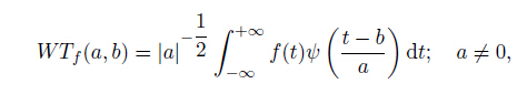
3.1 Data ProcessingSeismic data often contain various types of noise: some types of noise present a stable long period feature with strong amplitude or a short period feature of high frequency,whereas other types consist of random nonstationary signals; this variability introduces difficulties in discriminating the real seismic phases. Typically,the seismic signals are assumed to be stationary signals and are processed by removing the mean value,removing the trending variation,and performing signal tapering and high/low pass Fourier transform filtering. Nevertheless,we discovered that the OBS data signal-to-noise ratio was not improved after processing using the typical approach. Therefore,we use the Fourier transform first to perform high/low pass filtering and to perform bandpass filtering to suppress the stationary disturbances,and then use the time-frequency features of the wavelet transform to conduct threshold filtering in the wavelet domain to suppress the non-stationary noise. For the signal(or function)f(t)2L2(R),its continuous wavelet transform(CWT)is defined as
|
(1) |
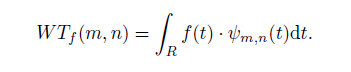
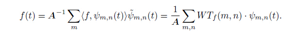
where a is a scaling factor that reflects the frequency change of the wavelet; b is a time factor that reflects the position of wavelet in the time window. The CWT of signal f(t)with ψ(t)is the transvection between f(t)and wavelet ψ(t). The CWT is a quantitative representation of similarity degree between the signal and wavelet series. The inverse transform of CWT is

|
(2) |
where 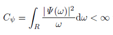
|
(3) |
The inverse DWT is
|
(4) |
The wavelet transform of all f(t)must satisfy the following condition:

|
(5) |
The discrete function series { m,n; m,n 2 Z} is the so-called “frame" in mathematics.
To explain the difference between one-dimensional Fourier transform filtering and wavelet transform filtering,we use the soft threshold method(Donoho,1995)on the collected data as an example. Fig. 2a shows three-components of the ZRT waveforms,which were cut from an earthquake event without filtering and lasted 150 s. From Fig. 2a,the radial component(red waveform)and the tangential component(green waveform)have strong low frequency features. Particularly in the tangential component,the effective wave is masked by noise.In addition,all the components are masked by many types of high frequency noise. Fig. 2b shows the signal after one-dimensional Fourier transform filtering with waveform analysis. To obtain a valid signal,we attempted to combine the following filters: high or low pass filter,bandpass filter,and notch filter. However,the result was not satisfactory. Fig. 2b shows that the noise is suppressed but the effective wave is lost at the same time.Further,the wave polarity is destroyed at some regions. Furthermore,we first used the Fourier transform to suppress the stationary noise,and then used the one-dimensional wavelet adaptive threshold filtering method to suppress the non-stationary noise. The result shown in Fig. 2c indicates that the latter approach is better at suppressing noise and maintaining the waveform. As a result,the signal-to-noise ratio is improved drastically.

|
Fig. 2 The comparison between Fourier transform filtering and wavelet transform filtering |
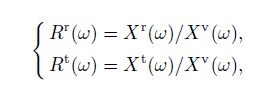
The steps of the extraction of the receiver functions from the actual records are as follows. First,three components of the seismic records are rotated,based on the earthquake azimuth relative to the station(as determined by the OBS compass),to obtain the radial component,the tangential component,and the vertical component. Next,the time domain signals are transformed into the frequency domain,and then the vertical component is used to divide two horizontal components for two receiver functions obtaining(Langston,1979):
|
(6) |
where Xr(ω),Xt(ω)and Xv(ω)are the radial,tangential and vertical component spectra,respectively,and Rr(ω)and Rt(ω)are the radial and tangential receiver functions spectra,respectively.
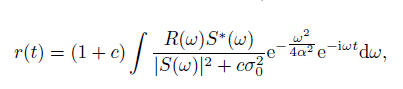
To ensure the stability of the receiver function calculation,a water level is introduced(Zhu and Kanamori,2000):
|
(7) |
where R(ω)is the horizontal component spectrum,S(ω)is the equivalent source spectrum represented by vertical component spectrum,S*(ω)is the complex conjugate of S(ω),
Finally,we obtained the receiver functions from the OBS observed data,as shown in Fig. 3. From these receiver functions,the P-s converted phases are easily recognized as the waves appearing several seconds after the P wave arrivals,indicating the relatively thin crust of the oceanic basin. Although some individual receiver functions extracted from various events at the same station have pronounced diversities that are not used in structure inversion,most receiver functions are quite consistent. These diversities possibly result from various aspects of the differences in the waves,such as focal depth,wave traveling path and event magnitude,and the seismic waves arriving at one station carry complicated random noise and path homogeneities. These problems remain to be further studied in the future. Because the individual receive functions have substantial differences,a single receiver function and stacked receiver functions are used in the inversion processing. The best fitted receiver function and the corresponding inverted model are selected as the final results.

|
Fig. 3 The teleseismic receiver functions extracted from station observations |
To overcome some of the issues of linear inversion methods,various nonlinear inversion techniques have been widely used,such as genetic algorithm(GA)(Shibutani et al.,1996),simulated annealing(SA)(Ingber et al.,1989),wavelet transformation(Wu et al.,2003),and the complex receiver function spectrum ratio(Liu and Li,1996). These methods are based on solving the global optimization problem by searching for the most optimized model from various models. We adopt the nonlinear inversion method known as the neighborhood algorithm(NA),which was proposed by Sambridge et al.(Sambridge,1999a; Sambridge,1999b; Sambridge,2001; Sambridge and Mosegaard,2002). This algorithm first preferentially samples a collection of models from a better fitting data domain and then determines the most optimized model in this collection. This procedure can improve the inversion precision compared with ordinary random searching to obtain a single optimal model. Correspondingly,the inversion code used in this study is NA-Sampler,in which the forward problem of the differential seismogram is based on the generalized reflection transmission matrix theory proposed by Kennett(1979). Furthermore,we use the H-k stacking method(Zhu and Kanamori,2000)to calculate the Moho depth and the Vp/Vs ratio as a test of the inverted model.
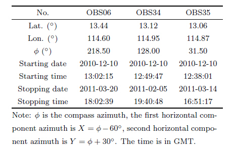
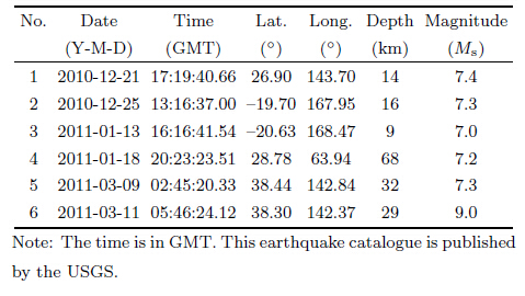
4 SEISMIC DATAAn active and passive synchronous seismic experiment was conducted using a 3D array of OBSs from Dec.2010 to Mar. 2011 at the abandoned spreading ridge of the southwestern subbasin in the SCS(Fig. 1)(Ruan et al.,2012). The passive data includes six earthquakes of magnitude ≥ Ms7.0 recorded by three Chinese made I-4C type broadband OBSs. The selected data have high signal-to-noise ratios and epicenter distances of 30° to 63°. The OBS station coordinates and the earthquake catalog are presented in Table 1 and Table 2,respectively.
|
|
Table 1 Coordinates and recording times of the OBS stations |
|
|
Table 2 Catalog of earthquakes (Ms ≥ 7.0) selected |
Using the above-described data processing,receiver function calculation and inversion methods,we obtained the lithospheric 1D S-wave velocity structure(beneath the seafloor)of three OBS stations at the southwestern subbasin in the SCS,as shown in Fig. 4. The results show that the uppermost crust is a 1~2 km thick low velocity layer,being especially thin at the OBS06 station,which is close to the ridge center axis. We propose that the shallow low velocity layer comprises sediments mixed with clastic rock from magma eruption that occurred after the ceasing of sea floor spreading. However,this layer is difficult to subdivide. Previous studies also indicated that,along both sides of the Changlong seamounts,the sediment thickness varies from 0.5 to 1 km at the central southwest subbasin and gradually increases northwestward and southeastward to 2~2.5km(Yao,1998). Seismic reflection profiles revealed that the spreading ridge has thick sediments(Gao et al.,2009). This prior observation is consistent with our results. The three 1D S-wave velocity models all indicate the presence of an abrupt velocity increasing discontinuity at a depth of 11~12 km,which is suggested to be Moho discontinuity. However,the active seismic 2D P-wave velocity profile indicated that the Moho depth of the same area is at approximately 10~12 km(below sea level)(Zhang,2013). Another 2D P-wave velocity profile also indicated that the Moho depth near our research area is at approximately 10 km(Pichot et al.,2014). Obviously,the data show that S-wave velocity model is different from the P-wave velocity model,the latter being shallower by 3~4 km. This is an important scientific discovery. We interpreted this result in two aspects. First,the Moho prefers to be a thick layer rather than a simple layer(Coleman,1977). Second,the S-wave velocity is more sensitive to melting and high temperature conditions than the P-wave velocity.
Note that the 1D S-wave velocity model beneath station OBS06 has a low velocity layer at depths of 6~12 km(above the Moho),different from the usual velocity downward increase,as observed at the other two stations. This difference may be explained by station OBS06 being closest to the spreading ridge axis(rift valley)where magma upwelled. Therefore,we suggest that this low velocity layer near the axis consists of melting magma or chamber. The numerical simulation of the thermodynamic structure showed that at depths of 8~12 km,the strain rate has an obvious change; in addition,at that depth,the oceanic crust is relatively weak and undergoes large tectonic deformation (Zhang and Shi,2008). Based on a 2D P-wave velocity model, Zhang(2013) suggested that there exist the combined effects of a detachment fault at the shallow crust and mantle melting at the lower crust.
Another remarkable velocity anomaly in the 1D models of OBS06 and OBS34 occurs at the depths from 17 km to 30 km,where the mantle has a small negative S-wave velocity gradient,whereas at the OBS35 station,at the depth of 26 km,the S-wave velocity decreases sharply. We speculate that a hot material supply source is present at the deep mantle beneath the spreading center axis. Correspondingly,previous studies have shown the following: 1)the SCS magmatism mainly occurred after the ceasing of seafloor spreading,and 2)the seamount age is young(14~3.5 Ma)(Yan et al.,2006; Wang et al.,2009). The heat flow measurements also showed that the southwest subbasin has a high heat flow value of 100~150 mW·m−2(Chen and Lin,1997;Zhang et al.,2001). As a result,we propose that,at the current tectonic and stress environment,although seafloor spreading has stopped,upper mantle melting still exists. This hypothesis merits future study because it has a great significance for our understanding of the deep hydrothermal state of the southwest subbasin in the SCS.

|
Fig. 4 Density diagram of the best 1000 S velocity models generated by the NA code |
We used the evaluation method of NA-Sampler to evaluate the above 1D S-wave velocity models. The Gauss factor is equal to 5,and the water level is equal to 0.001 in the forward calculation. The result is shown in Fig. 5. From Fig. 5,the receiver functions of all three models(blue solid line)are found to be very close to detected receiver functions(red solid line),especially within a few seconds after P wave. Pms and other Moho multiple wave are clear in the figure. The latter multiple waves are also clear. Thus,our result is reliable.

|
Fig. 5 Comparison between the observed receiver function and the predicted receiver function |
On the Moho discontinuity,many multiple P-s converted waves exist,for which the arrivals are very sensitive to the ratio variation of the Moho depth versus Vp/Vs. Thus,we can use the relationship between the travel times of multiple waves and the Moho depth along with the H-k stack procedure(Zhu and Kanamori,2000)to test the Moho depth inverted(Fig. 6). Within the depth range from 7 to 25 km,the Vp/Vs ratio ranges from 1.5 to 2 and the weighting factors are 0.7,0.2 and 0.1(Huang et al.,2011),the testing results of the grid searching stack shows that the Moho depths beneath OBS06,OBS34 and OBS35 are 12.5 km,10 km and 12.5 km,respectively,and the Vp/Vs ratios are 1.85,1.69 and 1.77,respectively. These results indicate that the obtained 1D velocity models have a good stability. Consequently,we obtained the crust mean Poisson ratios of 0.2936,0.2306 and 0.2656 for the three models of OBS06,OBS34,and OBS35,respectively,by using the following equation:

|
Fig. 6 The test results of the H-k stack procedure |
|
(8) |
where σ is the crustal Poisson ratio,and k is the Vp/Vs ratio.
6 CONCLUSIONSWe combined the use of the Fourier transform and the use of the wavelet transform to suppress the non-stationary disturbances in the OBS data successfully to acquire clear seismic phase records with high signal-to-noise ratio,and then conducted an analysis of the lithospheric structure of the southwest subbasin ridge in the SCS by using the receiver functions inversion technique for teleseismic data. The main conclusions of this study are as follows:
(1) The receiver functions inversion technique is feasible for use in analyzing OBS passive data,and suppressing the non-stationary disturbances is a key in data processing.
(2) The Moho depth of the southwest subbasin determined by S wave is 10~12 km(from the seabed)with a crust thickness of 6~8 km. This depth is 3 km deeper than the result determined by active seismic P-wave analysis. The shallow crust has a low velocity zone with a sediment thickness of 1~2 km; this crust possibly consists of sediments mixed with rock debris and fracture that resulted from magma eruption after sea floor spreading ceased.
(3) The models show that there is a low S-wave velocity zone at the depth of 6~12 km,just above the Moho discontinuity. We propose that the spreading center has a melting lower crust or magma chamber. At 17~30 km,the S-wave velocity is found to have a negative gradient. We speculate that a hot material supply source is present at the deep mantle beneath the spreading center axis. Although the seafloor spreading has stopped in the current tectonic and stress environment,upper mantle melting can still exist.
AcknowledgeWe thank all colleagues who joined this OBS experimental investigation of southwestern subbasin in the SCS in 2010–2011: Wu Z L,Dong C Z,Niu X W and Wei X D from the Second Institute of Oceanography,SOA,Zhu J J and Huang H B from the South China Sea Institute of Oceanology,Chinese Academy of Sciences,and Liang J W,Wang L J,Qiu M C,and Xu W F from Taiwan Ocean University. The investigation was conducted by separately using at different times in the following research vehicles: R/V “Fendou No.7",R/V “Kan 407",and R/V “hiyan No. 2". We used GMT software(Wessel and Smith,1995) for plotting some of the figures,the code provided by Lupei Zhu(Zhu and Kanamori,2000) for extraction of the receiver functions,and the code of NA-sampler(Sambridge et al.,2001,2002)for receiver functions inversion.
| [1] | Briais A, Patriat P, Tapponnier P. 1993. Updated interpretation of magnetic anomalies and seafloor spreading stages in the South China Sea:Implications for the tertiary tectonics of Southeast Asia[J]. J. Geophys. Res., 98 (B4): 6299–6328. |
| [2] | Chen X, Lin J F. 1997. The preliminary analysis about thickness and crustal age of the central basin of the South China Sea[J]. Acta Oceanologica Sinica (in Chinese), 19 (2): 71–84. |
| [3] | |
| [4] | Donoho D L. 1995. De-noising by soft-thresholding[J]. IEEE Transactions on Information Theory, 41 (3): 613–627. |
| [5] | Gao H F, Zhou D, Qiu Y. 2009. Relationship between formation of Zhongyebei basin and spreading of southwest subbasin, South China Sea[J]. Journal of Earth Science, 20 (1): 66–76. |
| [6] | Hao T Y, You Q Y. 2011. Progress of homemade OBS and its application on ocean bottom structure survey[J]. Chinese J. Geophys. (in Chinese), 54 (12): 3352–3361. DOI: 10.3969/j.issn.0001-5733.2011.12.033 |
| [7] | Huang H B, Qiu X L, Xu Y, et al. 2011. Crustal structure beneath the Xisha Islands of the South China Sea simulated by the teleseismic receiver function method[J]. Chinese J. Geophys. (in Chinese), 54 (11): 2788–2798. DOI: 10.3969/j.issn.0001-5733.2011.11.009 |
| [8] | Ingber L. 1989. Very fast simulated re-annealing[J]. Mathematical and Computer Modelling, 12 (8): 967–973. |
| [9] | Kennett B L N. 1979. Theoretical reflection seismograms for elastic media[J]. Geophysical Prospecting, 27 (2): 301–321. |
| [10] | Langston C A. 1977. The effect of planar dipping structure on source and receiver responses for constant ray parameter[J]. Bulletin of the Seismological Society of America, 67 (4): 1029–1050. |
| [11] | Langston C A. 1979. Structure under Mount Rainier, Washington, inferred from teleseismic body waves[J]. J. Geophys. Res., 84 (B9): 4749–4762. |
| [12] | Leahy G M, Park J. 2005. Hunting for oceanic island Moho[J]. Geophys. J. Int., 160 (3): 1020–1026. |
| [13] | Liu C G, Hua Q F, Pei Y L, et al. 2014. Passive-source ocean bottom seismograph (OBS) array experiment in South China Sea and data quality analyses[J]. Chinese Science Bulletin, 59 (33): 4524–4535. |
| [14] | Liu H F, Niu F L. 2012. Estimating crustal seismic anisotropy with a joint analysis of radial and transverse receiver function data[J]. Geophys. J. Int., 188 (1): 144–164. |
| [15] | Liu H Y, Niu X W, Ruan A G, et al. 2012. Analysis of seismic signals of ocean bottom seismometer[J]. Journal of Tropical Oceanography (in Chinese), 31 (3): 90–96. |
| [16] | Liu Q Y, Kind R, Li S C. 1996. Maximal likelihood estimation and nonlinear inversion of the complex receiver function spectrum ratio[J]. Chinese J. Geophys. (Acta Geophysica Sinica) (in Chinese), 39 (4): 500–511. |
| [17] | |
| [18] | Pichot T, Delescluse M, Chamot-Rooke N, et al. 2014. Deep crustal structure of the conjugate margins of the SW South China Sea from wide-angle refraction seismic data[J]. Marine and Petroleum Geology, 58 : 627–643. |
| [19] | Ruan A G, Li J B, Lee C S, et al. 2012. Passive seismic experiment and ScS wave splitting in the southwestern subbasin of South China Sea[J]. Chinese Science Bulletin, 57 (25): 3381–3390. |
| [20] | Sambridge M. 1999. Geophysical inversion with a neighbourhood algorithm-I[J]. Searching a parameter space. Geophys. J. Int., 138 (2): 479–494. |
| [21] | Sambridge M. 1999. Geophysical inversion with a neighbourhood algorithm-Ⅱ[J]. Appraising the ensemble. Geophys. J. Int., 138 (3): 727–746. |
| [22] | Sambridge M. 2001. Finding acceptable models in nonlinear inverse problems using a neighbourhood algorithm[J]. Inverse Problems, 17 (3): 387–403. |
| [23] | Sambridge M, Mosegaard K. 2002. Monte Carlo methods in geophysical inverse problems[J]. Reviews of Geophysics, 40 (3): 3–1. |
| [24] | Shibutani T, Sambridge M, Kennett B. 1996. Genetic algorithm inversion for receiver functions with application to crust and uppermost mantle structure beneath eastern Australia[J]. Geophysical Research Letters, 23 (14): 1829–1832. |
| [25] | Sun Z, Zhou D, Wu S M, et al. 2009. Patterns and dynamics of rifting on passive continental margin from shelf to slope of the Northern South China Sea:evidence from 3D analogue modeling[J]. Journal of Earth Science, 20 (1): 136–146. |
| [26] | Tian B F, Li J, Wang W M, et al. 2008. Crust anisotropy of Taihangshan mountain range in north China inferred from receiver functions[J]. Chinese J. Geophys. (in Chinese), 51 (5): 1459–1467. |
| [27] | Wang Y J, Han X Q, Luo Z H, et al. 2009. Late Miocene magmatism and evolution of Zhenbei-Huangyan Seamount in the South China Sea:evidence from petrochemistry and chronology[J]. Acta Oceanologica Sinica (in Chinese), 31 (4): 93–102. |
| [28] | Wessel P, Smith W H F. 1995. New version of the Generic Mapping Tools released[J]. EOS Trans. AGU, 76 (29): 329. |
| [29] | Wu Q J, Tian X B, Zhang N L, et al. 2003. Inversion of receiver function by wavelet transformation[J]. Acta Seismologica Sinica (in Chinese), 25 (6): 601–607. |
| [30] | Xu W W, Zheng T Y, Zhao L. 2011. Mantle dynamics of the reactivating North China Craton:Constraints from the topographies of the 410 km and 660 km discontinuities[J]. Sci. China Earth Sci., 54 (6): 881–887. |
| [31] | Yan P, Deng H, Liu H L, et al. 2006. The temporal and spatial distribution of volcanism in the South China Sea region[J]. Journal of Asian Earth Sciences, 27 (5): 647–659. |
| [32] | Yao B C. 1998. The discussion about seafloor spreading age of the South China Sea basin[J]. Geological Research of South China Sea (in Chinese), 10 : 23–33. |
| [33] | Zhang J, Xiong L P, Wang J Y. 2001. The characteristics and mechanism of geodynamic evolution of the South China Sea[J]. Chinese J. Geophys. (in Chinese), 44 (5): 602–610. |
| [34] | Zhang J, Shi X B. 2008. Numerical simulation of the lithospheric thermo-rheological structures and their rifting dynamics in the South China Sea. Li J B. Evolution of China's Marginal Seas and Its Effect of Natural Resources (in Chinese). Beijing:China Ocean Press[M]. : 283 -299. |
| [35] | |
| [36] | Zhu L P, Kanamori H. 2000. Moho depth variation in southern California from teleseismic receiver functions[J]. J. Geophys. Res., 105 (B2): 2969–2980. |