 2016, Vol. 59


2 Dept. of Science and Technology, Shenzhen Branch of CNOOC, Guangzhou 510240, China;
3 University of Chinese Academy of Sciences, Beijing 100049, China
In September to October of 2006, the Second Institute of Oceanography, State Oceanic Administration, and the South China Sea Institute of Oceanology, Chinese Academy of Sciences(SIO-joint-SCSIO)conducted a wide-angle reflected/refracted deep seismic profile(OBS2006-2)(Fig. 1)along the extinct spreading ridge in the Northwest Sub-basin of the South China Sea(SCS), for ascertaining its deep crustal velocity structure. This experiment deployed 12 German-made short-period auto-floating OBS(Li et al., 2007; Wu et al., 2008)and 11 of them were successfully recovered, resulting in a high recovery rate of 92%. First-hand data beneath the extinct spreading ridge were obtained, which provided key information for the extension of the northern continental margin of the SCS and the formation and evolution of the SCS(Ao et al., 2012).

|
Fig. 1 Bathymetric map and shaded-relief image of the Northwest and Southwest sub-basins of the South China Sea with 1000 and 3000-m isobaths (NWSB and SWSB respectively). Locations of the seismic lines OBS2006-2 and OBS973-3. The red, gray, black and pink circles, represent OBSs with abnormal data, with no data, lost stations, and normal stations, respectively |
However, some unexpected problems, such as the problems of data format or recording time, caused the failure of reading and utilizing the data in the data processing. OBS03 and OBS06 in the profile OBS2006-2 recorded abundant air-gun signals but failed to provide any effective seismic phase information. So they were abandoned in later simulation of the velocity structure(Ao et al., 2012). The absence of the data from OBS03, 06 and 09(Fig.1)increases the multi-solutions and uncertainty inevitably. Fig. 2 shows the ray-tracing and ray-coverage of PmP phase reflected from Moho and Pn phase refracted from uppermost mantle. Because of the abandonment of OBS03 and 06 and the loss of OBS09, PmP phase was obviously sparse in the range of 0~40, 100~120 and 260~310 km. Therefore, the morphology and depth of the Moho cannot be constrained effectively. Furthermore, due to the bad fitting degree of the Pn phase of OBS10(Fig. 2b)and the relatively big discrepancy between the theoretical travel-time and the actual travel-time(0.5 s), the Chi-Square of the Pn phase of the whole velocity model reached 3.075, much bigger than the ideal condition(about 1). In the further check-board test, the reconstruction of the output model to the input model was less-than-desirable(Fig. 2c)within poor ray-coverage regions mentioned above; while the consequences were just the reverse within good ray-coverage region, e. g. 170~210 km(between OBSs01 and 02), which suggests that the more the ray-coverage is, the better the constraint on velocity model and the more reliable the velocity structure becomes.

|
Fig. 2 (a) P-wave velocity model and travel-time simulation; (b) Observed travel-time curve (vertical bar) and calculated travel-time curve (dotted line) for PmP and Pn seismic phases; (c) Checkerboard test for velocity structure along the profile OBS2006-2; the grey OBS locations (OBS06, OBS03 and OBS09) mean that they are not used during the velocity simulation, T represents the absolute travel-time of seismic phases, PmP and Pn represent the wide-angle reflective arrivals and the refractive arrivals from Moho |
Given these problems of the velocity model of OBS2006-2 mentioned above, it would be important if the abnormal data collected by OBS03 and OBS06 can be fixed and provide any useful information to better constrain the deep crustal structure of line OBS2006-2. The method of processing OBS data is essential for a precise and reliable deep crustal structure. And the processing of abnormal data tests the strength and spirit of a research group. In addition, OBS data are very precious due to the high cost and arduous work offshore, especially when encountering bad weather like typhoon and depression. This survey was actually hit by the typhoon ‘Xangsane’(Ao et al., 2009), which not only gave a great physical challenge to the crew on board, but also caused the loss of an OBS worth as much as 250000 yuan(Fig. 1). So treasuring these data and making full use of them are the basic attitude for every marine geophysicist. This paper mainly focuses on reprocessing these 2 abnormal OBS’s data in profile OBS2006-2. We also obtained the seismic record section of OBS03 along the profile OBS973-3 with the same method, demonstrating that the reprocessing method for abnormal OBS data is reliable and effective, and would promote OBS survey and data processing level.
2 OBS DATA PROCESSING FOR SEDIS IVGeneral OBS data processing procedures(Fig. 3)have been discussed and applied widely(Zhao et al., 2004; Xia et al., 2007; Xue et al., 2008). Firstly, we convert the navigation data file to the standard UKOOA format file using C program-raw2ukooa, and raw OBS data(IMG format)to SAC format data using C program sedis2sac. Secondly, the received signals of each OBS station are checked with the seismic data analysis software SAC(Seismic Analysis Code)(William and Joseph, 1991). Air-gun signals with high Signal-Noise Ratio(SNR)are obtained after filtering, mean-removing, etc. Thirdly, with the shot time from UKOOA file, we use the C program sac2y to cut the air-gun signals out of the SAC format continuous data and convert them into an international standard SEGY format multi-trace data. Finally, the seismic processing software package SU(Seismic Unix)(Cohen and Stockwell, 1994)was employed to obtain the seismic record section(Fig. 4).

|
Fig. 3 Flow chart of data processing and format conversion for the SEDIS IV type of OBS |

|
Fig. 4 Seismic record section of normal OBS07 with the reduction velocity of 6.0 km·s−1 |
Generally, the cause for abnormal OBS data is either data format or recording time. First, we check the original data format and content of these 2 abnormal OBSs. The designed sampling interval for all the OBSs is 250 Hz by referring to the log. Original data is divided into blocks of one minute. Each one is 180080 bytes, whose beginning 80 bytes are the header recording the size of the header, sampling number, the number of components and the beginning time, and the later 18000 bytes are waveform data with 15000 sampling points(each taking 12 bytes)including 4 components(vertical component, horizontal component X, horizontal component Y and hydrophone component, each taking 3 bytes).
We wrote a C program sedisread to check the header of the original data, and found that the keywords such as the size of the header(80 bytes), sampling numbers(15000 bytes), the number of components(4 bytes), sampling intervals(4 ms)and the beginning time were all correct, which illuminates that these abnormal data can be read and have right data format.
3.1.2 Recording time information checkingNo problem occurred in the process when we converted original IMG data to SAC format data, and regular shooting signals can be seen by the SAC software. Unfortunately, the shot interval is not the designed interval and the air-gun signals appearing time does not consist with the time recorded in the UKOOA file(Fig. 5). So we preliminarily suspect the problem lies on the recording time, which results in asynchronization between waveform data clipped by the shot time and the shot signals. Consequently, nothing can be seen in the SEGY data, including the direct water wave arrivals(Pdw).

|
Fig. 5 The waveform graph of the first 9 shots in SAC format of the abnormal OBS06 |
Time information was stored in the 80 byte header which consists of 3 TimeDate fields: SampleTime, SedisTime and GPSTime. Each field contains second, minute, hour, day-of-week, day-of-month, month and year, and takes 8 bytes totally. We then rewrote the C program sedisread to read and output these 3 TimeDate fields of each minute, but they do not show any abnormal information and are not the causes of the abnormal data.
3.1.3 Adjacent OBSs comparison and analysisNo problem was found from the abnormal data themselves, so we turned to compare the abnormal OBSs with their adjacent OBSs. OBS07 was chosen to compare with abnormal OBS06 because we started shooting from the area nearby OBS08(Fig. 1). According to the shot time in UKOOA file, we found out the first 20 shots in OBS07(Fig. 6). The shot interval is 80 s from 1st to 6th shots and 120 s between 6th and 7th shots; then the shot interval became about 90 s from the 7th shot to the 20th. From the log, the first 7 shots are testing shots and they haven’t been recorded in UKOOA. UKOOA records from the 8th shot. A 26 s delay was found between the onset time in the waveform and the shot time in the 1st line of UKOOA(that is the 8th shot), which is equal to the travel time of Pdw from the firing shot to OBS07(the distance is 40 km and the assumed velocity in seawater is about 1.5 km·s-1). And there is a one-to-one correspondence between waveform data and UKOOA file after the 8th shot.

|
Fig. 6 Comparison of waveforms and shooting signal between instrument OBS07 (normal) and OBS06 (abnormal) in SAC format |
Unlike OBS07, due to the abnormal recording time, the air-gun signals cannot be found near the shot time in the waveform of OBS06. We eventually found the shot signals 13310 s later than expected after global search. Leaving out this time lag and aligning the waveform of OBS06 with OBS07(Fig. 6), we obtained 3 following understandings: ① Shot signals are regular and most of them are evenly spaced in time. But the shot interval between 6th and 7th shots is bigger than others, which proves that the shot signals, selected from OBS07 and 06, respectively, are from the same shots; ② The amplitude of shot signals in OBS06 is half of that in OBS07, in accordance with the fact that OBS06 is farther than OBS07 from these shots; ③ In OBS06, the shot intervals are larger than that of OBS07, and each shot has a certain amount of delay and gradually accumulated. The 1st shot signal of OBS06 is aligned with that of OBS07, then the delays become larger and larger for the following shot signals. This may be the real cause that we cannot find out any seismic phases when converting to SEGY format data.
After we found out the cause responsible for abnormal OBS06, we compared abnormal OBS03 with adjacent normal OBS02 using the same method and noticed that OBS03 had the same problem as OBS06-the delay of the air-gun signals and the stable increment of the interval between signals. We deduced that it is the built-in timers which are faster than normal that cause the delay of the air-gun signals. If the built-in timer is faster than normal(crystal oscillator frequency is faster), and the degree of fastness is constant(crystal oscillator frequency is invariant), the sampling interval(Delta)of the abnormal OBSs is no longer what we have designed(4 ms), but less than 4 ms. Such problem can be solved by special data processing method.
3.2 Solutions 3.2.1 Sampling interval(dt)adjustmentBased on the above analysis, we adjusted the dt in the software SAC manually to align the beginning and ending air-gun signals of the abnormal OBS data with adjacent normal OBS data. The dt that achieved the alignment is probably the true value. After constant adjustment and comparison, the adopted dt for OBS06 and OBS03 are 3.65708 ms and 3.65770 ms, respectively. We primarily fixed the abnormal data in the SAC format by adjusting dt and hoped that we could get seismic phases after converting the data to SEGY format. However, after the data were converted to SEGY format and plotted with a reduction velocity of 1.5 km·s-1, the phase with strongest amplitude Pdw didn’t show up in a horizontal line as expected. Instead, an inclined phase occurred with a rupture(Fig. 7). The amplitude of the phase indicated that it should be Pdw. But it obviously had a wrong apparent velocity and an unexpected rupture.

|
Fig. 7 Seismic record section of abnormal OBS06 without resampling with a reduction velocity of 1.5 km·s−1; other symbols are the same as in Fig. 4 |
Adjusting either the clipping window or the reduction velocity, the result didn’t change. In the end, we guessed that bugs existed in the converting C program sac2y. dt required in SEGY format is integral millisecond while dt is float now.
3.2.2 Resampling the SAC format dataWe rewrite a C program of interpolation-resampling based on the existing C program sedis2sac which reads every sample point of original data, demultiplexes and outputs them in 4 components of SAC format. The basic idea is that we first select a new integral dt(such as 4 ms), larger than the actual float dt, and then seek the location of each new data point in the original data(time axis). The value of the new point were determined by a linear interpolation between 2 original points before and after the new data point, and finally output all the data points from beginning to the end. Thus, we acquire the new SAC format data with integral dt. In the process of practical programming and debugging, we adopted a simpler algorithm: representing the value of the new point with the nearest original data point. Though the waveform details change a little bit, the characteristics of the shot signals remain unchanged. Fig. 8 is the sketch map of the 2 algorithms and shows the positions and waveform of the first dozen data points.

|
Fig. 8 Sketch map of data positions and waveforms before and after resampling and interpolation. The sampling intervals of original (blue) and interpolated (red) data are 3.5 ms and 4 ms, respectively; other symbols are the same as in Fig. 5 |
Converting the new SAC format data acquired after resampling and interpolation of SEGY data using sac2y, we finally obtained the seismic record section containing Pdw phase(Fig. 9). The consequences of the 2 interpolation methods are in agreement, indicating that the previous conjectures about sample interval and conversion program bugs are true. We can see that for both OBS03 and OBS06(Fig. 9), the direct water wave Pdw is in a horizontal line. The multiples of the Pdw gradually converge to Pdw as the offset increased. Pg and its multiples show up as downward sloping lines.

|
Fig. 9 Seismic record sections of (a) OBS03 and (b) OBS06 along the profile OBS2006-2 with the reduction velocity of 1.5 km·s−1 after linear interpolation; other symbols are the same as in Fig. 4 |
Supported by the national "973" project, another deep seismic exploration experiment OBS973-3 was carried out during March to April 2011(Fig. 1). A total of 20 OBSs, 8 SedisIV OBSs(No.01-08)from the Second Institute of Oceanography, State Oceanic Administration and 12 other type OBSs from the Institute of Geology and Geophysics, Chinese Academy of Sciences, were deployed at 20 km interval and 19 OBSs were recovered. The seismic source consisted of a four air-gun array with a total volume of 6000 in3 and was fired every 120 s, giving an average shooting interval of 300 m with the 5 knots ship speed(Qiu, 2011). Coincidentally, the same problem happened to the OBS03 in this OBS973-3 profile and the abnormal data were not used either(Lü et al., 2011).
When analyzing the abnormal data in profile OBS973-3, we found that the case is similar to OBS03 and OBS06 in OBS2006-2: ① They are all short period auto-floating SedisIV OBSs; ② Continuous shoot signals can be seen in the software SAC, but the shot interval is not equal to originally designed; ③ No seismic phase shows up in the seismic record section after conventional processing by the seismic processing software package SU, and these data were abandoned in the subsequent calculation and simulation(Lü et al., 2011; Ao et al., 2012; Lü, 2013).
Adopting the same method-adjacent OBS comparison and analysis, we tried to search the characteristic shot signal range in OBS02(or OBS04)that can be easily found in OBS03. OBS973-3 started shooting from north to south and the shooting signals in the end of the line were much clearer. Checking the UKOOA file, logs and waveform data, we eventually found a 400 minute blank zone without any shot between the shot 1754 and 1755 and regarded the zone as a reference for waveform comparison. Over a large number of sampling interval tests, we ultimately ascertained that the sampling interval of OBS03 was 3.65708 ms, which accords with that of OBS06 in OBS2006-2. So we conjectured that they may actually be the same instrument. Finally we obtained the seismic record section of OBS03 in OBS973-3(Fig. 10).

|
Fig. 10 Seismic record section of OBS03 along the profile OBS973-3 with the reduction velocity of 6.0 km·s−1; other symbols are the same as in Fig. 4 |
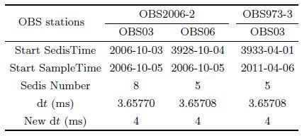
Each German SedisIV OBS has its own unique built-in Sedis Number. Noticing that the inside Sedis Numbers in OBS06 of OBS2006-2 and OBS03 of OBS973-3 both are 5 after checking the logs of the 2 cruises in 2006 and 2011, we affirmed that these 2 OBSs are the same instrument. In order to further ascertain above conjecture, we outputted and compared the Time-Date structure fields of the 3 abnormal OBSs data(Table 1)using C program sedisread time, and found that the time span of TimeDate structure field of OBS06 in OBS2006-2 and OBS03 in OBS973-3 are both 5 years, which confirms the guess again.
|
|
Table 1 Comparisons of information of abnormal stations along the profiles OBS2006-2 and OBS973-3 |
After the abnormal data processing above, we can get the following enlightenment: ① The judgment of abnormal data. We firstly convert the data according to conventional procedure of data processing(Fig. 3), then obtain the seismic record section and examine whether there are seismic phases, if not, we can predict that it is abnormal data. ② Check the abnormal OBS data itself, such as the data format and parameters in the converting procedures. ③ Adjacent OBSs comparison and analysis. Find out the causes responsible for the abnormality and the rule of the abnormal data by the method mentioned above and then, try to solve the problem and reuse the data. ④ Software SAC is a critical means to do waveform comparison and we should take full advantage of it. The success of the abnormal data reprocessing not only provides ideas for original data decoding but improves the universality of the decoding programs as well.
4 SEISMIC PHASE IDENTIFICATION AND WORK PROSPECTSFor deep crustal seismic phase identification, we plotted the seismic record sections of OBS03 and OBS06 along the profile OBS2006-2 with the reduction velocity of 6.0 km·s-1 and noticed that they contained a lot of useful information about deep crustal structure(Fig. 11a, Fig. 12a). In order to validate these seismic phases, we employed Rayinvr software(Zelt and Smith, 1992)to conduct ray-tracing and travel-time simulation based on the velocity model of Ao et al.(2012). Following seismic phases in OBS03 are recognized: Pg refracted from crust with large offset that can be traced up to -80 km; PmP, which is reflected from Moho interface and present as hyperbolic curve with large apparent velocity, its left branch offset is -38~-80 km and 35~78 km for the right; and Pn refracted from the uppermost mantle immediately follow the left PmP and extend from -80 km to -93 km, which are all accordant with the COT(Continent Ocean Transition)geologic setting(Fig. 11). So does OBS06(Fig. 12). At present, we just have completed primary forward simulation based on 893 newly-picked Pg travel-time phases, 578 PmP and 43 Pn. We have reasons to believe that the reliability and resolution of the velocity model will be improved tremendously with the increasing seismic phases.

|
Fig. 11 (a) Seismic record section of OBS03 (vertical component) along the profile OBS2006-2 with the reduction velocity of 6.0km/s; (b) The fit between observed travel-time curves (color vertical bars) and calculated traveltime curves (black lines) of P-wave; (c) P-wave velocity model and ray-tracing simulation; ray paths in different colors correspond to different seismic phases in (b), respectively; other symbols are the same as in Fig. 4 |

|
Fig. 12 (a) Seismic record section of OBS06 (vertical component) along the profile OBS2006-2 with the reduction velocity of 6.0 km·s−1; (b) The fit between observed travel-time curves (color vertical bars) and calculated traveltime curves (black lines) of P-wave; (c) P-wave velocity model and ray-tracing simulation ray paths in different colors correspond to different seismic phases in (b), respectively; other symbols are the same as in Fig. 4 |
Next, we will add these 2 abnormal OBS data and conduct the reprocessing of OBS2006-2 based on previous work(Ao et al., 2012)to acquire a more accurate velocity model. After that, we will set about the joint forward and inversion of P wave and S wave to obtain the S wave velocity model, Vp/Vs ratio, Poisson’s ratio and the lithology, providing information for understanding the formation and evolution mechanism of the Northwestern sub-basin.
ACKNOWLEDGMENTSThis work was supported by the National Natural Science Foundation of China (91428204, 91028002, 41306046, 41276049). Thanks for the assistance of the crew members of the R/V Fendou 7 from Shanghai Offshore Petroleum Bureau on OBS2006-2. We are grateful to the technical staff from SCSIO and the crew members of the R/V Shiyan2, all of whom took part in the field work at sea during OBS973-3. We are also grateful to Prof. Aiguo Ruan for providing original logs of OBS2006-2. Thanks for the help from Jian Wang and Jinhu Chen on data processing.
| [1] | Ao W, Zhao M H, Ruan A G, et al. 2009. The impaction of typhoon on seafloor ambient noise by analyzing the OBS recording data[J]. Journal of Tropical Oceanography (in Chinese), 28 (6): 61–67. |
| [2] | Ao W, Zhao M H, Qiu X L, et al. 2012. Crustal structure of the Northwest Sub-Basin of the South China Sea and its tectonic implication[J]. Earth Science-Journal of China University of Geosciences (in Chinese), 37 (4): 779–790. |
| [3] | Cohen J K, Stockwell J W. 1994. The SU user's manual. Center for Wave Phenomena, Colorado School of Mines, 1-40. |
| [4] | Lü C C, Hao T Y, Qiu X L, et al. 2011. A study on the deep structure of the northern part of southwest subbasin from ocean bottom seismic data, South China Sea[J]. Chinese J. Geophys. (in Chinese), 54 (12): 3129–3138. DOI: 10.3969/j.issn.0001-5733.2011.12.013 |
| [5] | Lü C C. 2013. The rift to drift development of the southwest sub-basin and its continental margin, South China Seaan integrated geophysical study from MCS/OBS experiments[Ph. D. thesis][M]. Beijing: University of Chinese Academic of Sciences . |
| [6] | Li X Y, Wu Z L, Xue B, et al. 2007. Short-period auto-floating ocean bottom seismometer and its operational experiences[J]. Journal of Tropical Oceanography (in Chinese), 26 (5): 35–39. |
| [7] | Qiu X L. 2011. The report of supplementary OBS survey in the south of Xisha for Project 973(in Chinese). |
| [8] | William C T, Joseph E T. 1991. SAC-Seismic Analysis Code Users Manual[J]. Lawrence Livermore National Laboratory, Livermore, CA : 1–153. |
| [9] | Wu Z L, Ruan A G, Li J B, et al. 2008. New progress of deep crust sounding in the mid-northern South China Sea using ocean bottom seismometers[J]. South China Journal of Seismology (in Chinese), 28 (1): 21–28. |
| [10] | Xia S H, Qiu X L, Zhao M H, et al. 2007. Data processing of onshore-offshore seismic experiment in Hongkong and Zhujiang River Delta region[J]. Journal of Tropical Oceanography (in Chinese), 26 (1): 35–38. |
| [11] | Xue B, Ruan A G, Li X Y, et al. 2008. The seismic data corrections of short period auto-floating ocean bottom seismometer[J]. Journal of Marine Sciences (in Chinese), 26 (2): 98–102. |
| [12] | Zelt C A, Smith R B. 1992. Seismic traveltime inversion for 2-D crustal velocity structure[J]. Geophysical Journal International, 108 (1): 16–34. |
| [13] | Zhao M H, Qiu X L, Xia K Y, et al. 2004. Onshore-offshore seismic data processing and preliminary results in NE South China Sea[J]. Journal of Tropical Oceanography (in Chinese), 23 (1): 58–63. |