 2016, Vol. 59


2 National Geophysical Observatory at Mengcheng, Bozhou Anhui 233527, China
The use of dispersion data from earthquake surface waves and ambient noise to invert for underground velocity structure is a very important and mature method(e.g., Shapiro et al., 2005; Yao et al., 2008), but this method has certain limitations. The surface wave phase or group velocity at a specified period is sensitive to the underground structure within a certain depth range. As the period becomes longer, the sensitive depth increases and the sensitive depth range becomes broader, resulting in the decreased depth resolution of deeper structures(Xu et al., 2007). Besides, it is not easy to obtain the accurate velocity structure for the top several kilometers of the shallow crust as high quality short period dispersion data are difficult to obtain. By improving the resolution of velocity structure from a few hundred to a few thousand meters of the uppermost crust, we will be able to better relate the geological feature of the Earth’s surface to the structure anomaly and evolution process of deep crust, and it is also of great significance to understand and predict earthquake-induced geological hazards as well as for exploration of mineral and oil and gas resources.
For the fundamental mode Rayleigh wave, the phase of its radial component is different from its vertical one by 90°. The amplitude ratios of those two components of Rayleigh wave, which is called as the ZH ratio, have a close relationship with the shallow underground structure. ZH ratio is a function of frequency, and for the vertically transverse isotropic and radially varying layered Earth model, ZH ratio is only affected by the mechanical properties of the underground medium at the receiver site and has nothing to do with other parameters(e.g., seismic source)(Tanimoto and Alvizuri, 2006). With the increasing number of broadband seismic stations and the improvement of data measurements and processing techniques, there are more and more studies about ZH ratio. Tanimoto and Alvizuri(2006)searched for the fundamental mode Rayleigh waves from continuous noise signals using the 90° phase difference between the radial and vertical components, then computed the ZH ratios and inverted for the shear velocity structure of shallow crust. Tanimoto and Rivera(2008)used numerical methods to obtain the depth sensitivity kernels of ZH ratio for intermediate to long period(20~250 s)surface wave records. Compared to the dispersion curve of the fundamental mode Rayleigh wave, they found that ZH ratio is more sensitive to shallow structures. Yano et al.(2009)inverted for the crustal and upper mantle structure beneath different GEOSCOPE stations using ZH ratio of intermediate to long period Rayleigh waves. Tanimoto et al.(2013)developed a new method to compute ZH ratios from continuous noise signals.
Both the surface wave dispersion curve and ZH ratio can be used to invert for the underground velocity structure, but their depth sensitivity ranges are different and ZH ratio can make up the limitation of dispersion data that can not constrain the shallow crust structure accurately. In a very early study, Boore and Toksöz(1969)conducted joint inversion of dispersion and ZH ratio. Lin et al.(2012)combined intermediate to long period(24~100 s)ZH ratios and dispersion curves within the period band of 8~100 s to invert for the crustal and upper mantle structure of western America. Lin et al.(2014)computed the short to intermediate period(8~24 s)ZH ratios beneath a station from the cross-correlation of three-component ambient noise data. They can be used to better invert for the 3D velocity structure of the crust and upper mantle of western America when combined with ZH ratio data within 24~100 s and phase velocity dispersion data from 8 to 100 s that are obtained from earthquake records. All of these joint inversions of ZH ratio and dispersion data are based on the linearized least squares inversion method and need to compute the ZH ratio and its sensitivity kernels. Chong et al.(2015)proposed a joint inversion method for surface wave dispersion curve and ZH ratio based on the Simulated Annealing Algorithm. They conducted random searches directly in the model space to obtain the global optimal model without computing the sensitivity kernels.
This paper proposes a joint inversion method that is based on Neighborhood Algorithm(NA)(Sambridge, 1999a, 1999b)using surface-wave dispersion curve and ZH ratio and then obtains the errors and resolution of the inversion results as well as the correlation among different parameters through Bayesian analysis. We first demonstrate the reliability of the joint inversion method based on NA through synthetic tests, and then apply the joint inversion method to real seismic data.
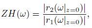
2 RAYLEIGH WAVE ZH RATIO AND DEPTH SENSITIVITY KERNEL OF DISPERSIONWe define the ZH ratio as the ratio of vertical to horizontal amplitude of the fundamental mode Rayleigh wave at the surface of the Earth(z = 0), that is
|
(1) |
where ω is frequency, |r1(ω|z)| and |r2(ω|z)| are Rayleigh-wave eigenfunction values at the depth z and frequency ω(Aki and Richards, 1980), respectively.
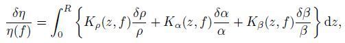
Surface-wave dispersion is important for inversion of crustal and upper mantle 3D shear wave velocity structures. With regard to linear inversion methods, it is essential to compute depth sensitivity kernels of phase or group velocity to S-wave velocity, P-wave velocity and density at different frequencies. For ZH ratio, Boore and Toksöz(1969)suggested that the medium mechanical parameters that affect ZH ratio involve P-wave and S-wave velocity and medium density, while the Q value can be neglected. Among all of those parameters, ZH ratio is most sensitive to the variations of shear wave velocity. The equation of depth sensitivity kernel of Rayleigh wave ZH ratio(or phase velocity)at a specified frequency f can be expressed as follows
|
(2) |
where η is ZH ratio(or phase velocity c), ρ is density, α is P-wave velocity, β is S-wave velocity, and δp(p = ρ, α, β)represents the perturbation of density, P-wave velocity or S-wave velocity, respectively. All of these parameters(p and δp)are functions of depth z. Kp is called as the sensitivity kernel and is a function of frequency and depth.
Figure 1 presents the depth sensitivity kernels of Rayleigh-wave ZH ratio and phase velocity to structural parameters at three different periods for a 1D layered model with crustal thickness of 45 km. It can be seen clearly that for ZH ratio and phase velocity their depth sensitivity kernels are very different, especially to S-wave velocity. Compared with phase velocity, ZH ratio is more sensitive to shallower structures, about half of the sensitive depth for phase velocity at the same period(Tanimoto and Rivera, 2008), and ZH ratio has the largest sensitivity at the surface of the Earth. Thus ZH ratio data can be used to invert for much shallower S-wave velocity structure than dispersion data of the same frequency band. Rayleigh-wave dispersion is also sensitive to crustal P-wave velocity and density, so does ZH ratio to shallow crustal density, but the sensitivity of it to P-wave velocity is quite low.

|
Fig. 1 Depth sensitivity kernels at different periods for Rayleigh wave fundamental mode phase velocity (a) and ZH ratio (b) to Vs, Vp and density, respectively |
As the depth sensitivity kernel of ZH ratio is different from that of surface-wave dispersion, and ZH ratio constrains shallow structure better, we can combine it with dispersion data to conduct joint inversion in order to constrain the crustal velocity structure more accurately(e.g., Lin et al., 2012). In this paper, we develop a joint inversion algorithm for ZH ratio and dispersion data based on the Neighborhood Algorithm(NA)(Sambridge, 1999a, 1999b).
3.1 Neighborhood Algorithm(NA)Neighborhood Algorithm is a kind of inversion method based on global search and it involves two stages. In the first stage, it searches acceptable(good)models in the model space using special geometric partition method(Sambridge, 1999a), and then in the second stage, Bayesian analysis is conducted to the models generated in the former stage. The degree of deviation of 1-D marginal posterior probability density functions(PPDFs)with respect to the Gaussian distribution can be used to judge whether the inversion result is reliable, and we can represent the uncertainty of models by the width(that is, standard deviation)of the 1-D PPDF. 2-D marginal PPDFs can be used to estimate the trade-off between two different model parameters, and the more concentrated to be circular the distribution is, the smaller the trade-off is. 1-D and 2-D PPDFs are both useful tools to estimate the resolution and uncertainty of model parameters(Sambridge, 1999b).
3.2 Inversion Based on the Theoretical ModelIn order to verify the superiority of joint inversion of dispersion and ZH ratio data to inversion of dispersion alone, we conduct an NA inversion test with data generated from forward modeling of a theoretical model.
3.2.1 Construction of the theoretical model and data preparationThe theoretical model we construct includes two parts(i.e., crust and upper mantle)from 0 km to 310km in the upper mantle followed by a half space layer. The crust is divided into four layers and its thickness is 45 km. The Vp/Vs value is 1.9 in the first layer and 1.7 in the rest three layers. We first set the shear-wave velocity(Vs)values in these four crustal layers and compute the P-wave velocity(Vp)of the corresponding layer according to the Vp/Vs value, and then we can obtain the density value from P-wave velocity through an empirical formula(Brocher, 2005). The setting of upper mantle velocity is directly from the ak135 model(Kennett et al., 1995)and its depth extends from 45 km to 310 km(Table 1). According to this model we adopt the method of Herrmann and Ammon(2004)and obtain 31 Rayleigh-wave phase velocity dispersion data(period band 5~150 s)and 26 ZH ratio data(period band 5~120 s). All of these data(noise-free)will be used in the following NA inversion test.
|
|
Table 1 The reference values and their perturbation ranges for 10 parameters in the NA inversion |
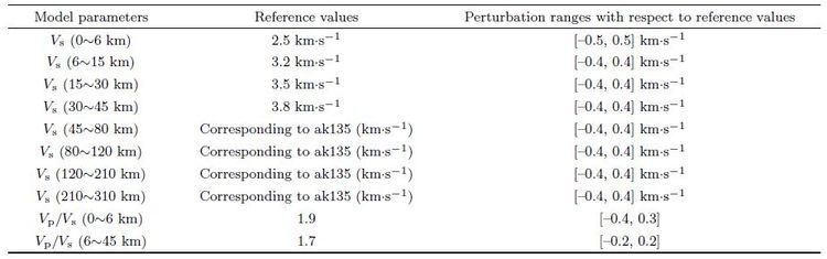
Table 1 presents the 10 parameters we plan to invert for with NA, involving the eight shear wave velocity values of four crustal layers and four upper mantle layers as well as the two Vp/Vs values of the first crustal layer(0~6 km)and the rest three crustal layers as a whole(6~45 km). We give the variation range for each Vs parameter with respect to the theoretical model as the reference(see Table 1). It is worthy to be noticed that each of the four layers of upper mantle contains several thinner layers that is directly from the ak135 model, and for all of these thinner layers within a common thick layer in the new generated model, the values of the model parameters will vary systematically with respect to the reference values. Besides, as the depths of discontinuities cannot be constrained very well by surface wave data and there are always large trade-offs between adjacent layers(e.g., Yao et al., 2008), we usually do not invert for layer thickness(or depth of discontinuity).
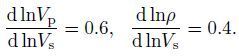
The S-wave velocity of each layer will be generated by NA, and then we can obtain the corresponding P-wave velocity from Vp/Vs values if they are also model parameters or the empirical formula(Brocher, 2005). Then the density values are computed through the empirical equation(Brocher, 2005). While this empirical equation is not suitable for the upper mantle part, we employ the variation relationship of P-wave velocity and density relative to S-wave velocity(Masters et al., 2000; Yao et al., 2008)as
|
(3) |
The L1-norm misfit function is used during the inversion process:
|
(4) |
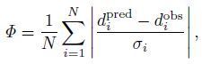
where N is the number of data of ZH ratio and phase velocity dispersion within a specific period band(here N = 57), dipred and diobs are the data computed from the theoretical models and observations at the ith period, respectively, and σi stands for the standard error of observed data at the ith period and here σi is set to be 0.01 diobs .
In consideration of the reliability and the rate of convergence of inversion, 20 new models(Ns = 20)are generated at each iteration after trial and error. Combined with former generated models, the model space will be partitioned again to produce a new distribution of Voronoi cells. Then 10 best cells(Nr = 10)will be chosen from all the cells and 20 new models will be generated again. In this way, we repeat the procedure until convergence of NA searches. After that, we will perform Bayesian statistic analyses on all of the models generated before to obtain the posterior mean and standard error(corresponding to the 68% confidence interval)of each model parameter.
Figures 2-4 show the direct inversion results of the 10 parameters(Table 1). In Fig. 2 the thin black solid line represents the posterior mean model while the dashed line gives the optimum one. The optimum model agrees very well with the theoretical model, while the posterior mean model has certain deviation with the theoretical model for some parameters. The posterior mean shear-wave velocity of the lower crust is higher than that of the true model by about 0.12 km·s-1 while the posterior mean S-wave velocity of the uppermost mantle is lower than that of the true model by about 0.18 km·s-1 due to the trade-off of S-wave velocities between the fourth(lower crust)and fifth(uppermost mantle)layers around Moho(see the 2-D PPDFs in Fig. 4).

|
Fig. 2 Shear-wave speed model of crust and upper mantle obtained from the one-step joint inversion (Left), comparison of phase velocity dispersion (Middle) and ZH ratios (Right) calculated from the statistical posterior mean, optimum and theoretical models, respectively |

|
Fig. 3 1-D marginal posterior probability density functions (PPDFs) shown as the shaded area of the 10 model parameters from the joint inversion of the dispersion and ZH ratio data |

|
Fig. 4 2-D marginal posterior probability density functions (PPDFs) of the 10 model parameters from the joint inversion of the dispersion and ZH ratio data |
As Fig. 3 shows, though the 1-D PPDFs present Gaussian distribution and most of the posterior mean values of model parameters are consistent with those of the true model, the standard error of the inverted model is slightly larger because of the broader range of PPDF. If there are many parameters during the global search of NA, the inversion result may be unstable due to significant trade-off between these parameters so that the search is likely to be trapped into regions of local minima and the posterior mean model we finally get will deviate from the true model.
Thus we attempt to implement the inversion in two steps. In the first step only the S-wave velocities of a number of crust and upper mantle layers are inverted for, which are totally 8 parameters here, that is, the S-wave velocities of four crustal layers and four upper mantle layers(as shown in Table 1). After a relatively reliable model of upper mantle is determined, we start the second step inversion for 7 parameters, which are values of Vs of four crustal layers(same as step 1)and one upper mantle layer(45~310 km)as well as values of Vp/Vs of the first crustal layer(0~6 km)and the rest three crustal layers(6~45 km). The reference model of step 2 is the result of step 1, that is, the posterior mean Vs model of the crust and upper mantle from step 1 is set as the initial reference model of step 2. In step 2 the number of inversion parameters of upper mantle decreases from four to one, which means that Vs of upper mantle(Moho-310 km)will vary as a whole with respect to the shear-wave velocity model obtained in step 1 in this depth range. We hope to constrain the crustal shear-wave velocity structure better and the Vp/Vs values that are not inverted for in step 1 through the variation of inversion parameters.
The results of two-step NA joint inversion are shown in Figs. 5-7. In Fig. 5 we compare the posterior mean model from NA inversion with the theoretical model and find that they are very close to each other. And the error of the final obtained model is small compared to the one-step inversion result. Besides, the values of surface wave dispersion and ZH ratio computed from the posterior mean model nearly coincide with the theoretical ones(Fig. 5), which verifies the correctness of our posterior mean model and the reliability and accuracy of NA joint inversion. Obviously the two-step joint inversion is superior to the single step inversion(Figs. 2-4).

|
Fig. 5 Shear-wave speed posterior mean model (solid line) and theoretical model (dashed line) of the crust and upper mantle obtained from the two-step joint inversion (Left), comparison of phase velocity dispersion (Middle) and ZH ratios (Right) calculated from the posterior mean and theoretical models, respectively. |

|
Fig. 6 1-D marginal posterior probability density functions (PPDFs) of the seven model parameters from the dispersion and ZH ratio two-step joint inversion (black solid lines and the shaded area) in comparison with the results from dispersion data only (dashed lines). In each plot, the solid or dashed vertical line shows the parameter value of the posterior mean model for the joint inversion or inversion with dispersion data only, respectively |

|
Fig. 7 2-D marginal posterior probability density functions (PPDFs) between different model parameters from the NA joint inversion based on the synthetic data from the theoretical model |
The shaded area of Fig. 6 shows the 1-D marginal PPDFs, and the posterior mean values of all the model parameters are indicated by the positions of the vertical black lines while the maximum likelihood model can be obtained from the peak of these 1-D distributions(Sambridge, 1999b). Compared to the one-step results(Fig. 3), Fig. 6 shows that the 1-D marginal PPDFs of these inversion parameters are basically in Gaussian distribution with narrow variation ranges, which demonstrate small standard deviations and high resolution of the model parameters. Except for Vs, the values of Vp/Vs are also consistent with the theoretical values. The standard error of Vp/Vs from 6 km to Moho is obviously larger than that from 0 km to 6 km, implying that the joint inversion constrains Vp/Vs in the shallow crust better.
Figure 7 shows the 2-D marginal PPDFs of different model parameters. Compared with the one-step inversion results in Fig. 4, the contour lines of 2-D marginal PPDFs for different Vs parameters are nearly circular with smaller radius, that is, more concentrated distribution. So the Vs values of the four crustal layers can be constrained very well with weak correlation between each other. From Fig. 7, Vs of the first crustal layer(0~6 km)nearly has no correlation with Vp/Vs of the same layer but has obvious negative correlation with the Vp/Vs of the depth range from 6 km to Moho. Meanwhile, the Vp/Vs of the first crustal layer whose error is apparently small has little correlation with that of the rest crustal layers, which is consistent with analysis of the 1-D marginal PPDFs in Fig. 6.
By comparison, the two-step joint inversion has better inversion results with higher resolution and we will adopt this new method to real data for the inversion process.
3.2.3 Inversion with Rayleigh wave dispersion data onlyIt is common to invert for the underground velocity structure with dispersion data. Here we carry out the same inversion process as in Section 3.2.2 but only use 31 dispersion data. As the dashed vertical lines show in Fig. 6, the posterior mean model we get after the inversion is far from the theoretical model. The 1-D PPDFs after inversion have wider distribution, especially for Vs of the first two crustal layers(0~6 km and 6~15 km). Besides, some parameters have multiple peaks, which indicate strong non-uniqueness of the model parameters through inversion using just dispersion data. By comparison, we decide to adopt the optimal model, which has the minimum data fitting error instead of the posterior mean model from inversion(as shown in Fig. 8). Fig. 8 clearly indicates that although the optimum model can give almost perfect fit to the dispersion data, the predicted ZH ratios are still very different from the theoretical ones. This illustrates that there are certain limitations in traditional inversion methods using just dispersion data, which cannot constrain some model parameters very well and results in larger uncertainties of inversion results for some parameters.

|
Fig. 8 Inversion results from the dispersion data only. In the left plot, the black solid line gives the best fitting model from the NA inversion. Other symbols are similar as in Fig. 5 |
There always exist larger errors in actual measurements of ZH ratios from either earthquake surface waves or ambient noise. Tanimoto and Rivera(2008)suggested that the error distribution is stable and can be dealt with statistical methods. In order to reduce the error, we set some selection criteria during the process of extracting amplitude ratios from earthquake Rayleigh waves. For instance, we require that signal to noise ratio(SNR)of Rayleigh waves must be larger than 10, the phase difference between radial and vertical components of Rayleigh waves should be around 90°, and the obviously abnormal measurements of ZH ratio should also be removed, etc. Fig. 9 shows the ZH ratio distributions at the period of 45 s and 85 s, respectively, and both of them are approximately in Gaussian distribution. The ZH ratios we finally obtained are generally consistent with those computed from the existing crust and upper mantle model(Yao et al., 2010), which demonstrates the reliability of ZH ratio measurement used in this inversion.

|
Fig. 9 The histograms of ZH ratios (close to Gaussian distribution) at different periods (45 s and 85 s) of the KMI station measured from earthquake surface waves. The black vertical line in each figure represents the mean value of ZH ratios at the corresponding period, respectively |
There are total 39 dispersion measurements in the period range of 10~150 s involved in the joint inversion, which come from the phase velocity interpolation results at the location of the Kunming station from Rayleigh wave tomography of southeast Tibetan plateau(Yao et al., 2010). For ZH ratio, there are total 29 observed data within the period range of 25~110 s.
4.2 Reference ModelThe reference model of NA joint inversion involves crust and upper mantle and the rest part below 310 km is set as the half space. The crust is divided into three layers(0~15 km, 15~30 km, 30~45.554 km)whose Vs values are 3.3 km·s-1, 3.6 km·s-1, 3.8 km·s-1 from top to bottom, respectively. In reference of Yao et al.(2010), the depth of Moho discontinuity is set to 45.554 km and the upper mantle part from 45.554 km to 310 km is still taken from the ak135 model.
4.3 Steps and Results of NA Joint InversionWe follow the same inversion process and take the same value of Ns and Nr as in the previous synthetic tests. In the first step, we invert for 7 parameters of shear wave velocity for 3 crustal layers and 4 upper mantle layers(Moho-80 km, 80~120 km, 120~210 km, 210~310 km). In the second step, we invert for 6 parameters, that is, Vs of 3 crustal layers and 1 upper mantle layer(Moho-310 km)as well as the Vp/Vs of the first crustal layer(0~15 km)and the rest crustal layers as a whole(15 km-Moho). The reference model in the second step is selected from the posterior mean model in the first step. During the second step inversion, the Vs values will be adjusted on the basis of Vs model from the first step while the emphasis is put on the inversion of Vp/Vs.
The joint inversion results are showed in Figs. 10-12. In Fig. 10, the final obtained model is shown as the thick black solid line and the phase velocity dispersion and ZH ratios computed from this model are roughly within the error range of observed data. When the period is above 140 s, there are larger differences between the calculated and observed data, probably due to the existence of large errors in the long period dispersion measurements, which makes the inversion of deep upper mantle structure not very reliable. In Fig. 11, the 1-D marginal PPDFs of all the inversion parameters are approximately in narrow Gaussian distribution, indicating high resolution for the model parameters. It should be pointed out that there are two peaks in the 1-D marginal PPDF of Vp/Vs from 15 km to Moho and one has apparently higher probability than the other. Instead of taking the posterior mean value(between the two peaks)as some other parameters, we set the value of Vp/Vs that corresponds to the higher peak(the maximum likelihood value)to be the ultimate inversion result. Besides, the Vp/Vs values for the designed two crustal layers are both around 1.72, which is generally consistent with the existing Poisson’s ratio values of this area computed from receiver functions(Huang et al., 2008; Xu et al., 2009). This demonstrates that joint inversion of ZH ratio and dispersion data can be used to obtain Vp/Vs ratios(or Poisson’s ratios)for layered crust. Fig. 12 gives the contours of 2-D marginal PPDFs of every two parameters, which are more spread out for the real data results compared with the synthetic test results(see Fig. 7). However, the innermost contour line(red)that corresponds to the 60% confidence level is nearly circular with very small radius.

|
Fig. 10 Shear-wave speed model of crust and upper mantle beneath the station KMI obtained from real seismic data through joint inversion (Left), comparison of the phase velocity dispersion obtained from inversion and the observed dispersion data (Middle), same as the Middle plot but for ZH ratios (Right). In the left plot, the black solid line gives the final posterior mean model after inversion with the gray area showing its standard error, and the dashed line and the dot dashed line is the reference model for the first stage and second stage NA inversion, respectively. In the middle and right plots, the dots with the error bar are the observed data; the dotted line and the triangles are the synthetic data from the reference model in the first and second stage NA inversion, respectively; the solid line shows the synthetic data computed from the final posterior mean model after inversion |

|
Fig. 11 1-D marginal posterior probability density functions (PPDFs) of the model parameters from the joint inversion of real data (similar as Fig. 6). Except the bottom right plot, the vertical line in each plot represents the posterior mean model; for the bottom right plot, the vertical line shows for the model with the most likelihood |

|
Fig. 12 2-D marginal posterior probability density functions (PPDFs) of the model parameters from the joint inversion of real data (Similar as Fig. 7) |
It is notable that in spite of very casual selection of the initial reference model in the first step, the final results are nearly not affected if proper variation ranges of parameters are given. The forward ZH ratio and dispersion data from the model obtained in the first step of inversion(also the reference model of the second step)are already very close to the observed values, while in the second step, the forward results from the inversion model generally fall into the error range of the observed data. From Fig. 10 we can see that although there are large differences between the forward data from the initial reference model(dashed line)and the final inverted model(thick solid line), relatively accurate results can still be obtained from a worse initial model after the two-step joint inversion process, which strongly verifies the robustness of our joint inversion method.
5 DISCUSSION AND CONCLUSIONIt is very common to investigate the underground velocity structure using phase velocity dispersion curves. But the resolution within some depth ranges is insufficient and the constraint on the shallow crust is weak. The depth sensitivity kernels of ZH ratio are independent of those of phase velocity, and for the same period the depth range of sensitivity of ZH ratio is significantly different from that of phase velocity and much closer to the shallower crust. The combination of these two datasets can greatly improve the resolution of shallow crustal structure.
In this paper we propose a joint inversion method using dispersion and ZH ratio data based on NA. Compared with one-step inversion, we find that two-step inversion is more stable and can constrain the shearwave velocity structure of crust and upper mantle as well as the Vp/Vs values of layered crust more accurately. Through synthetic tests, we found that when there are too many parameters to be inverted for in the onestep process, the statistical posterior mean model may be far away from the theoretical model and the search process is easily to be trapped into local minima, although the optimum model we obtain is very close to the theoretical model. Besides, the joint inversion is obviously superior to inversion with dispersion data alone and can constrain the model parameters better as well as can reduce the error of inversion. Later we apply this two-step joint inversion method to the real data and obtain a more reliable model of the crustal velocity structure beneath the Kunming station. Besides, the joint inversion based on NA can better analyze model errors and the correlations between different parameters through the PPDFs.
Previous relevant studies either did not invert for the Vp/Vs value or find strong trade-offs between Vp/Vs and density. In this paper, we adopt a more proper empirical formula of P-wave velocity and density(Brocher, 2005)in order to constrain the Vp/Vs value better without inverting for density. From the real data inversion result of the Kunming station, the Vp/Vs values of the layered crust through the joint inversion are generally consistent with the average Poisson’s ratio from the previous receiver function method, implying that the combination of dispersion and ZH ratio can provide constraints on the Poisson’s ratio of the layered crust independently, which can provide new constraints for understanding composition and physical properties of the crust at different depths.
In addition, we divide the crust into three layers that have approximately the same thickness during the inversion with real seismic data. While in the synthetic test, the crust has four layers, with the top 15 km crust being divided into two layers(0~6 km and 6~15 km)since ZH ratio has strong constraints on the shallow crust structure in particular for short periods ZH ratio data. The beginning period of data in the theoretical test is 5 s and all of the four crustal layers are constrained very well. In real inversion, the beginning periods of phase velocity and ZH ratio data are 10 s and 25 s, respectively, thus it is difficult to invert for the top several kilometers structure of the shallow crust. As for earthquake surface waves, the beginning period of ZH ratio we measure is usually above 20 s(Lin et al., 2012). In order to study the velocity structure of the shallow crust better, we can also obtain the short-period ZH ratios through continuous ambient noise signals(Tanimoto et al., 2013)or the cross-correlations of ambient noise(Lin et al., 2014).
To sum up, the joint inversion of dispersion and ZH ratio is definitely superior to inversion with dispersion data alone, but the resolution of joint inversion is also affected by several factors like data quality, period range, etc. Besides, in view of the lack of constraints on interfaces with surface wave dispersion and ZH ratio, we do not invert for the depth of Moho or other discontinuities. We can probably get better results about discontinuities if receiver function data are added. Though surface wave dispersion and receiver functions are both sensitive to the S-wave velocity structure, they do have different strengths. Surface wave dispersion curve can reveal the variations of S-wave velocity structure while receiver function is relatively poor at constraining the absolute S-wave velocity but has a unique advantage in determining the depths of interfaces. Thus the combination of surface wave dispersion and receiver function information can provide more reliable shear wave velocity structure(Hu et al., 2005, Liu et al., 2010). In recent years, the joint inversion of surface wave dispersion and receiver function is widely used in the studies of crustal and upper mantle velocity structures(e.g., Hu et al., 2005, Liu et al., 2010). The purpose of joint inversion is to combine the strengths of different datasets. Therefore, the joint inversion of surface wave dispersion, ZH ratio, and receiver function for the crust and upper mantle velocity structures can more accurately constrain the model and reduce uncertainties of inversion results. This is also the hot research direction at present.
ACKNOWLEDGMENTSWe thank two reviewers for their constructive comments on our manuscript paper. We also thank Dr. Weisen Shen for providing the automated surface wave time-frequency analysis program that is used in the measurement of seismic surface wave amplitude. This study is supported by the National Natural Science Foundation of China (41574034), China National Special Fund for Earthquake Scientific Research in Public Interest (201508008), and the Fundamental Research Funds for the Central Universities in China (WK208cjg-59-02-13953).
| [1] | Aki K, Richards P G. 1980. Quantitative Seismology, Vol. 1:Theory and Methods[M]. San Francisco: WH Freeman and Company . |
| [2] | Boore D M, Toksz M N. 1969. Rayleigh wave particle motion and crustal structure[J]. Bulletin of the Seismological Society of America, 59 (1): 331–346. |
| [3] | Brocher T M. 2005. Empirical relations between elastic wavespeeds and density in the Earth's crust[J]. Bulletin of the Seismological Society of America, 95 (6): 2081–2092. |
| [4] | Chong J J, Ni S D, Zhao L. 2015. Joint inversion of crustal structure with the Rayleigh wave phase velocity dispersion and the ZH ratio[J]. Pure and Applied Geophysics, 172 (10): 2585–2600. |
| [5] | Herrmann R B, Ammon C J. 2004. Computers programs in seismology, surface waves, receiver functions and crustal structure, version 3.30. Department of Earth and Atmospheric Sciences. Saint Louis University. |
| [6] | Hu J F, Zhu X G, Xia J Y, et al. 2005. Using surface wave and receiver function to jointly inverse the crust-mantle velocity structure in the West Yunnan area[J]. Chinese J. Geophys. (in Chinese), 48 (5): 1069–1076. |
| [7] | Huang J P, Chong J J, Ni S D, et al. 2008. Inversing the crustal thickness under the stations of China via H-Kappa method[J]. Journal of University for Science and Technology of China (in Chinese), 38 (1): 33–40. |
| [8] | Kennett B L N, Engdahl E R, Buland R. 1995. Constraints on seismic velocities in the earth from traveltimes[J]. Geophysical Journal International, 122 (1): 108–124. |
| [9] | Levshin A L, Pisarenko V F, Pogrebinsky G A. 1972. On a frequency-time analysis of oscillations[J]. Annales Geophysicae, 28 (2): 211–218. |
| [10] | Lin F C, Schmandt B, Tsai V C. 2012. Joint inversion of Rayleigh wave phase velocity and ellipticity using usarray:Constraining velocity and density structure in the upper crust[J]. Geophysical Research Letters, 39 : L12303. |
| [11] | Lin F C, Tsai V C, Schmandt B. 2014. 3-D crustal structure of the western United States:Application of Rayleigh-wave ellipticity extracted from noise cross-correlations[J]. Geophysical Journal International, 198 (2): 656–670. |
| [12] | Liu Q Y, Li Y, Chen J H, et al. 2010. Joint inversion of receiver function and ambient noise based on Bayesian theory[J]. Chinese J. Geophys. (in Chinese), 53 (11): 2603–2612. |
| [13] | Masters G, Laske G, Bolton H, et al. 2000. The relative behavior of shear velocity, bulk sound speed, and compressional velocity in the mantle:implications for chemical and thermal structure.//Earth's Deep Interior:Mineral Physics and Tomography From the Atomic to the Global Scale.Washington D C, American Geophysical Union, 63-87. |
| [14] | Sambridge M. 1999a. Geophysical inversion with a neighbourhood algorithm-I[J]. Searching a parameter space. Geophysical Journal International, 138 (2): 479–494. |
| [15] | Sambridge M. 1999b. Geophysical inversion with a neighbourhood algorithm-Ⅱ[J]. Appraising the ensemble. Geophysical Journal International, 138 (3): 727–746. |
| [16] | Shapiro N M, Campillo M, Stehly L, et al. 2005. High-resolution surface-wave tomography from ambient seismic noise[J]. Science, 307 (5715): 1615–1618. |
| [17] | Tanimoto T, Alvizuri C. 2006. Inversion of the HZ ratio of microseisms for S-wave velocity in the crust[J]. Geophysical Journal International, 165 (1): 323–335. |
| [18] | Tanimoto T, Rivera L. 2008. The ZH ratio method for long-period seismic data:sensitivity kernels and observational techniques[J]. Geophysical Journal International, 172 (1): 187–198. |
| [19] | Tanimoto T, Yano T, Hakamata T. 2013. An approach to improve Rayleigh-wave ellipticity estimates from seismic noise:Application to the Los Angeles Basin[J]. Geophysical Journal International, 193 (1): 407–420. |
| [20] | Xu G M, Yao H J, Zhu L B, et al. 2007. Shear wave velocity structure of the crust and upper mantle in western China and its adjacent area[J]. Chinese J. Geophys. (in Chinese), 50 (1): 193–208. |
| [21] | Xu Q, Zhao J M, Cui Z X, et al. 2009. Structure of the crust and upper mantle beneath the southeastern Tibetan Plateau by P and S receiver functions[J]. Chinese J. Geophys. (in Chinese), 52 (12): 3001–3008. |
| [22] | Yano T, Tanimoto T, Rivera L. 2009. The ZH ratio method for long-period seismic data:Inversion for S-wave velocity structure[J]. Geophysical Journal International, 179 (1): 413–424. |
| [23] | Yao H J, Beghein C, Van Der Hilst R D. 2008. Surface wave array tomography in SE Tibet from ambient seismic noise and two-station analysis-Ⅱ[J]. Crustal and upper-mantle structure. Geophysical Journal International, 173 (1): 205–219. |
| [24] | Yao H J, Van Der Hilst R D, Montagner J P. 2010. Heterogeneity and anisotropy of the lithosphere of Se Tibet from surface wave array tomography[J]. Journal of Geophysical Research, 115 (B12). DOI: 10.1029/2009JB007142 |