 2016, Vol. 59


2. Earthquake Administration of Hebei Province, Shijiazhuang 050021, China
Precise information on seismometer orientation is of great significance in the study of seismic anisotropy,measurements of surface wave frequency dispersion,receiver function analysis and focal mechanism determination using waveform data. Borehole seismic observation can effectively reduce the impact of ground noise, and improve the observation accuracy of microseismic events. At present,there are more than 180 3-component borehole seismic stations in China,with instrumentation varying from very broadb and to short period sensors. Orienting equipment such as gyroscope is generally used in the installation of a borehole seismometer to determine the bearings of the two horizontal components. Sensor orientation was not measured with a gyroscope for some station during their installation,but was estimated by indirect methods after installation.
Due to the difference in accessibility between deep borehole and surface stations,it is difficult to measure the actual horizontal azimuth of a borehole seismometer directly using a gyroscope or other equipments. Normally teleseismic events or microtremor records are needed to detect the azimuth of a borehole seismometer. The seismograms recorded by borehole and surface seismometers are different in frequency spectrum (Xu et al., 1991) . Therefore,it is still challenging to obtain accurate instrumental azimuth with teleseismic and microtremor records. The noise shows some frequency dependent coherence,especially for the long period oceanic microseism. The correlate radius defined as the largest distance that the recorded noises exhibit some coherence thus depends on frequency. Generally,it increases to the range of a few kilometers at low frequency band (Bormann,2002) . Peterson (1993) studied earth's noise around the globe, and proposed a noise model that has been widely used. This noise model shows large noise peaks in period range from 1 to 10 s. The corresponding noise is generally believed to arise from the interaction between ocean and continent, and is relatively stable. Lacoss et al. (1969) conducted a detailed study on the microseism, and concluded that the noise in the frequency b and from 0.2 Hz to 0.3 Hz consists of both body and surface waves,with high-mode Rayleigh waves being the major component. Aster and Shearer (1991) proposed a method to determine the sensor orientation of a borehole station using the first P-wave arrivals of local earthquakes. They show that the method can reach a precision of 5°. Niu and Li (2011) used the teleseismic P-wave polarity to calculate the horizontal azimuths of all seismic stations within China, and found that some of the deep borehole seismometers have problems related to the azimuth polarity. There are studies (e.g.,Bormann,2002; Xie,2014) using correlation between collocated surface and borehole sensors to determine the sensor orientation of a borehole seismometer. These studies involved installing a 3C seismometer at the surface near the borehole station. By comparing the surface and borehole records from the same earthquakes,in principle,it is possible to determine the azimuth of the two horizontal component of the borehole sensor from the component orientation of the surface sensor. However,there's no detailed analysis related on the reliability and accuracy of this method.
Here we applied a correlation-based analysis method using a reference sensor to estimate component azimuth of a borehole seismometer. We applied this technique with a set of reference seismometers that have very different frequency b and , and are located at a wide range of distance from the target station. The results were used to evaluate the robustness of the measurements,as well as precision estimates. We further compared the borehole records with the set of surface records in order to see how robust the estimated component azimuth of the borehole sensor based on each surface seismometers. This comparison allows constraining the measurement precision and accuracy and thus provides basis for the next stage analysis in determining sensor orientation of the borehole seismometers across China.
2 METHODOLOGY OF SEISMIC SENSOR ORIENTATION DETERMINATION 2.1 Correlation AnalysisBy using the correlation analysis method we can obtain statistical relationship between two stochastic variables. To determine the component orientation of a surface or borehole seismometer,we employ a reference station method. We first installed a surface reference station, and measured the sensor orientation with a gyroscope. We refer the station with unknown component azimuths as the target station. In order to search for the sensor orientation of the target station,we rotated its 3C seismograms by assuming a component azimuth and rotate the seismograms to the NS,EW directions. We then correlate the NS,EW seismograms with the seismograms of the reference stations. We then varied the assumed azimuth in the range of 0~360°, and selected the sensor orientation that has the largest cross correlation coefficient.
2.2 Seismic Observation SimulationThe seismogram is the convolution of the source signal and the impulse response of a seismometer. The simulation program calculates the seismogram based on the given source signal. In general,we can obtain middle,long, and short period seismograms from a broadb and records by convolving the corresponding instrument response. The convolution can be performed either in frequency or time domain,which is widely studied (e.g.,Li,1992; He et al., 1997; Liu et al., 1997; Jin et al., 2004; Xie,2014) . In this paper we employed Fourier analysis,i.e.,computing the convolution within the frequency domain. For the instrument response,we only considered the low frequency part of the seismometers,while the high frequency part (digitizer) was ignored.
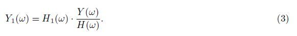
Assuming a broadb and system,if the observation is y (xt) ,source signal is x (xt) ,the system impulse response is h (xt) ,then in time domain we can have

In frequency domain we have

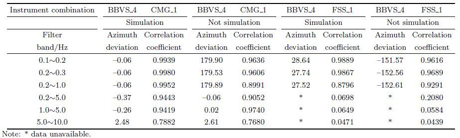
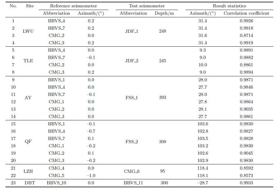
The filtering parameters were selected based on the global earth noise model given by Peterson (1993) and the results from real data calculation. The power spectrum density curves of the background noise recorded at site AY are shown in Fig. 1. The frequency b and information of BBVS-60,CMG-40T,CMG-40TDE is shown in Table 2. From the figure we can see that within 1~10 s there exists a peak for both the broadb and and short-period seismometers. For the frequency b and above 1 Hz,the noise levels recorded at the surface BBVS-60,CMG-40T,CMG-40TDE sensors are higher than the high level in the global noise model. However,the borehole sensor FSS-3DBH at the same site shows a noise level below the high end of the global earth noise model,indicating that the borehole observation can significantly reduce short-period noise. For better illustration,we separate the 0.1~10 Hz frequency range into several narrow frequency b and s. For each frequency b and ,we computed two sets of cross correlation coefficients. The first sets were derived from the convolution method described in the previous section, and the second sets were calculated from b and pass filtering. In the frequency b and 0.2~0.3 Hz,we found that there is a 180° phase difference between the two sets of cross correlation coefficients, and the first set cross correlation coefficients generally have a higher magnitude. These features are clearly shown in Table 1,Figs. 2 and 3. From the Fig. 4,we can find the origin of the 180° phase difference. For the BBVS-60 and CMG-40T broadb and seismometers,at the frequency b and of 0.2~0.3 Hz,the phase-frequency curve only changes slightly around 0°. For example,the phase angles at 0.2 Hz is 7° and 13° for the BBVS-60 and CMG-40T,respectively. In contrast,the short-period sensors,CMG-40TDE and FSS-3DBH,have a phase response that changes rapidly between 0.2 and 0.3 Hz. For example,CMG-40TDE and FSS-3DBH have a phase angle of 146° and 146°,respectively at frequency of 0.2 Hz. The phase difference at 0.2 Hz between the two broadb and (BBVS-60 and CMG-40T) and the two short period (CMG-40TDE and FSS-3DBH) is therefore greater than 130°,which is well above 90°, and consequently there is a polarity difference between the broadb and and short period seismograms. Therefore,when pairing seismograms for computing cross-correlation,we use the recordings directly between very broadb and and broadb and stations,but use the convolution records for very broadb and ,broadb and and short-period pairs. All the seismometers listed in Table 1 were installed with a gyroscope in aligning their component orientations. For the surface BBVS-60 broadb and seismometers and CMG-40TDE short-period seismometers combination (S/N: G10821VS,T4U81) ,the computed angle difference of component azimuth is very small in the frequency range below 5 Hz. The corresponding cross correlation coefficients are all above 0.94 (Table 1) . For the surface broadb and BBVS-60 and the borehole short-period FSS-3DBH sensor pair (S/N: G10821VS,889) ,the recorded ambient noise in the frequency range above 1Hz has almost no correlation. In the frequency range of 0.2~0.3 Hz,the records at the two sensors seem to have relatively good correlation. This is likely caused by the high attenuation at high frequencies when surface noise penetrates to subsurface. Therefore the high-frequency noise recorded at a deep borehole sensor is generally much lower than that in the surface data. Meanwhile,the ocean microseism within 0.2~0.3 Hz contains mostly high-mode Rayleigh waves (Lacoss et al., 1969) ,which can penetrate to a depth roughly equivalent to half of the wavelength. The borehole sensor is located within the half-wavelength depth range,thus its Rayleigh-wave dominant records showed a good correlation with surface records. The low correlation between borehole and surface records in high frequency has been noticed by many studies. For example,the surface data of earthquakes usually contain more information than their deep borehole records (Xu et al., 1991) . High frequency is generally lacking in borehole data (Wei and Li, 1990) . The detailed frequency response of the seismometers shown in Table 1 can be found in Table 2.

|
Fig.1 Power spectral density curve of background noise at AY (determined by detecting seismometer) |

|
Fig.2 Microtremor records of G10821VS and T4U81 without simulation (a) Original waveform of G10821VS seismometer at EW component; (b) Original waveform of T4U81 seismometer at EW component; (c) Waveforms after filtering and without rotation; (d) Waveforms with filtering and rotating; (e) Correlation coefficient map of full azimuths; (f) Correlation coefficient map, near the optimal rotation azimuth. |

|
Fig.3 Microtremor records of G10821VS and T4U81 with simulation (a) Original waveform of G10821VS seismometer at EW component; (b) Original waveform of T4U81 seismometer at EW component; (c) Waveforms after filtering and simulating without rotation; (d) Waveforms with filtering, simulating and rotating; (e) Correlation coefficient map of full azimuths; (f) Correlation coefficient map, near the optimal rotation azimuth. |

|
Fig.4 Frequency characteristic curves of detecting seismometers at AY |
| Table 1 The correlation analysis of different frequency band microtremor records with simulation and without simulation |
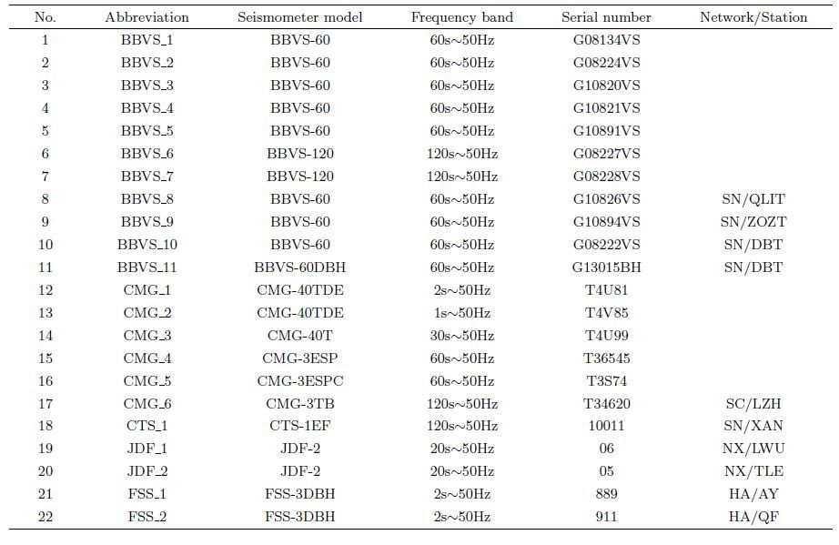
| Table 2 Information on the seismometers used in this work |
Based on the observed noise peak in 1~10 s from the global noise model derived by Peterson (1993) and the analysis described in the previous section (Section 2.3) ,we selected the frequency b and of 0.2~0.3 Hz for all the following data analysis. We noticed that this frequency b and is slightly different from those used by Lüet al. (2007) and Xie (2014) . The results on azimuthal direction in this paper are the arithmetic average of two horizontal components.
3.1 DataWe have used multiple surface sensors to calculate the component azimuth of a borehole station using reference stations that are located from a few hundred meters to a few kilometers from the borehole station. The locations of the stations are measured with a GPS system. The calibration of surface instruments was conducted at three experiment locations,which are QLIT,XAN and ZOZT. At each location,we chose more than 2 sites for conducting the experiments. Among the multiple sites,we chose one to be the major site and installed very broadb and ,broadb and and short period sensors at the site. We selected 6 deep borehole stations,LWU,TLE,AY,QF,LZH, and DBT for measurements. The sensors at these 6 sites range from very broadb and ,broadb and to short period. Details in frequency responses of these sensors are shown in Table 2.
If there is a housed pier at the experiment site,we generally install the seismometers on the pier. Otherwise,we install the sensor to a vault outside a building. We usually place a marble or granite plate at the base of the vault, and place the sensor on top of the plate. We use a gyroscope to align the sensor. We further cover the sensor with a hard case, and finally bury the instruments completely,which can reduce the noise associate with wind,airflow and rains. We kept continuous records for more than 24 hours and selected 24-hour records for performing the correlation analysis. The results can be considered the sampling average of the 24 recording.
The seismometers,BBVS-120,BBVS-60,BBVS-60DBH and FSS-3DBH seismometers,together with the digitizers,EDAS-24IP and EDAS-24GN,are manufactured by the Beijing Gangzhen instrument Ltd. The very broadb and sensor CTS-1EF is made by the Wuhan Liquan Seismic Observation Technology Co. Ltd, and the CMG-3TB,CMG-3ESP,CMG-3ESPC,CMG-40T,CMG-40TDE seismometers are made by the UK Guralp Company. JDF-2 is a short-period seismometer made by the Beijing Seismic Science and Technology Center. The CMG-40TDE is a short-period digital seismometer with a S/N T4U81 and T4V85,which is a sensor-digitizer all-in-one seismometer that has a sampling rate of 100 sps,minimum phase filtering, and a convert coefficient 3.178 μV/count. The EDAS-24IP digitizer has a sampling rate of 100sps,minimum phase filtering, and a convert coefficient 1.589 μV/count,while the EDAS-24GN digitizer has a sampling rate of 100 sps equipped with minimum phase filtering and a convert coefficient 1.192 μV/count.
3.2 Surface Sensor CalibrationThe first experiment location QLIT has 3 sites,QLIT,Q01 and Q02. Among them,QLIT was installed on the bedrock; Q01 and Q02 are placed on soil sediments. Site Q01 were equipped with two BBVS-60 broadb and seismometers with a SN G08224VS and G10820VS,respectively. The measured sensor azimuths of the north component are 1.1° and 0.3°,respectively. At the site Q02,we installed a total of four seismometers. A BBVS-60 broadb and sensor (SN: G10891VS) and a CMG-40T broadb and sensor (SN: T4U99) are oriented in 0.3° clockwise from the north direction. One BBVS-60 broadb and sensor (SN: G10821VS) and a short-period sensor (CMG-40TDE with a SN of T4U81) were installed to align to 29.7° clockwise from the north. At QLIT,we only installed one broadb and sensor (BBVS-60 with a SN number of G10826VS) that is oriented at 0.3° clockwise from the north. Except for the G10826VS sensor that was connected to the EDAS-24IP digitizer,all the other sensors are paired with the EDAS-24GN digitizer.
The distance between the QLIT and Q01 sites is ~2249 m,with an elevation difference of 130 m. We used the G10826VS sensor at the QLIT site as the reference seismometer. We then computed the component azimuths of the two broadb and sensors at the Q01 site. The calculated sensor azimuths of the G08224VS and G10820VS sensors are -1.0° and -2.3°,respectively. They are slightly different from the gyroscope-measured azimuths,1.1° and 0.3° for the G08224VS and G10820VS,respectively. The differences are -2.1° and -2.6°, and the corresponding cross correlation coefficients are 0.8672 and 0.8694,respectively.
The distance between QLIT and Q02 is 2541 m, and the elevation difference is 140 m. Again we employed the G10826VS sensor at the QLIT site as the reference seismometer, and measured the component azimuths of the four sensors at the site Q02,G10821VS,T4U81,G10891VS and T4U99. The estimated azimuth directions are 28.0°,28.5°,-2.8°,-2.8°,respectively. The corresponding azimuths measured by the gyroscope are 29.7°,29.7°,0.3°, and 0.3°,respectively,resulting in a difference of -1.7°,-1.2°,-3.1°, and -3.1°. The corresponding cross correlation coefficients are 0.8301,0.8053,0.8326 and 0.8166,respectively.
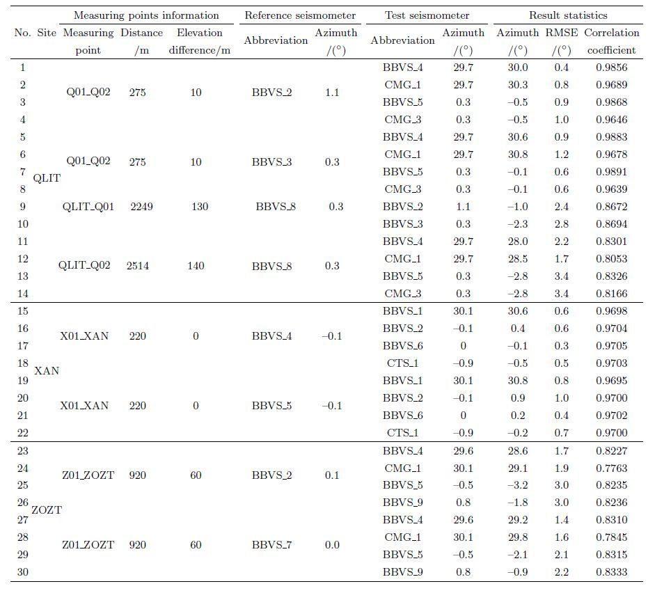
The distance between Q01 and Q02 is 275 m,with an elevation difference of 10 m. We took the sensor G08224VS at the Q01 site as the reference station, and computed the component azimuths of the four stations at the Q02 site (G10821VS,T4U81,G10891VS and T4U99) . The estimated component azimuths of these four sensors are 30.0°,30.3°,-0.5°, and -0.5°,respectively. Compared to their azimuths measured by the gyroscope,which are 29.7°,29.7°,0.3°, and 0.3°,respectively,the differences are 0.3°,0.6°,-0.8°, and -0.8°. The correlation coefficients are 0.9856,0.9689,0.9868,0.9646,respectively. Meanwhile,if we use the other broadb and sensor G10820VS at Q01 as the reference station,then the estimated component azimuths of the four sensors,G10821VS,T4U81,G10891VS and T4U99 at the site Q02 are 30.6°,30.8°,-0.1°, and -0.1°. The corresponding errors are 0.9°,1.1°,-0.4°, and -0.4°, and the cross correlation coefficients are 0.9883,0.9678,0.9891 and 0.9639,respectively.
The second experiment location is XAN,which has 2 sites,X01 and XAN. Both are situated on bedrocks. At the site XAN,we installed three sensors,a BBVS-60 broadb and sensor (SN: G08224VS) ,a BBVS-120 type very broadb and sensor (SN: G08227VS) , and another CTS-1EF type very broadb and sensor (SN: 10011) along the north direction. The measured direction with a gyroscope is -0.1°,0.0° and -0.9°,respectively. We also installed another BBVS-60 type broadb and sensor (SN: G08134VS) in the direction of 30° from the north,with a gyroscope-measured direction being 30.1° clockwise from north. At the X01 site,we installed two BBVS-60 type broadb and sensors (SNs: G10821VS and G10891VS) in the north direction,with a true direction of -0.1° and -0.1°,respectively. The very broadb and CTS-1EF sensor (SN: 10011) at the XAN site is connected to a EDAS-24IP digitizer,while the other sensors are recorded by a EDAS-24GN digitizer.
The X01 and XAN are separated by ~220 m,with a roughly similar elevation. We used one of the broadb and sensors (G10821VS) at X01 as the reference station, and then computed the sensor orientations of the four seismometers at the XAN,G08134VS,G08224VS,G08227VS and 10011. Their calculated component azimuths are 30.6°,0.4°,-0.1° and -0.5°,respectively. Compared with the gyroscope-measured azimuths 30.1°,-0.1°,0.0°,-0.9°,the differences are 0.5°,0.5°,-0.1° and 0.4°,respectively. The corresponding cross correlation coefficients are all very high,which are 0.9698,0.9704,0.9705 and 0.9703,respectively. We further used the other broadb and sensor (G10891VS) as the reference stations, and the calculated component azimuths of the four stations at XAN are 30.8°,0.9°,0.2° and -0.2°,respectively. These resulting errors are 0.7°,1.0°,0.2° and 0.7°, and the corresponding cross correlation coefficients are 0.9695,0.9700,0.9702 and 0.9700.
The third experiment location is ZOZT,which has 2 sites,Z01 and ZOZT. Z01 is located on sediment,while ZOZT is based on bedrocks. At the ZOZT site,we installed two BBVS-60 type broadb and seismometers (SNs: G10891VS and G10894VS) ,with a gyroscope-measured direction of -0.5° and 0.8°,respectively. We also installed another BBVS-60 (SN: G10821VS) and a short-period sensor (CMG-40TDE,SN: T4U81) along the N30°E direction. The actual directions are 29.6° and 30.1°,respectively. At the site Z01,we installed a BBVS-60 (SN: G08224VS) broadb and sensor and a BBVS-120 very broadb and seismometer (SN: G08228VS) . Their estimated azimuths are 0.1° and 0.0° clockwise from the north. The BBVS-60 (SN: G10894VS) at the site ZOZT was connected to a EDAS-24IP digitizer and the sensors were paired with a EDAS-24GN digitizer.
The two sites of Z01 and ZOZT are separated by ~920 m, and have an elevation difference of 60 m. We first used the G08224VS broadb and sensor at the site Z01 as the reference station, and computed the component azimuths of the four sensors at the site ZOZT,which are 28.6°,29.1°,-3.2° and -1.8° for the G10821VS,T4U81,G10891VS, and G10894VS,respectively. Compared to the gyroscope measurements,which are 29.6°,30.1°,-0.5° and 0.8°,the corresponding differences are -1.0°,-1.0°,-2.7° and -2.6°,respectively. The computed cross correlation coefficients are 0.8227,0.7763,0.8235 and 0.8236. Next,we used the other very broadb and sensor (G08228VS) as the reference station. The estimated component azimuths of the four sensors at the site ZOZT (G10821VS,T4U81,G10891VS, and G10894VS) are 29.2°,29.8°,-2.1° and -0.9°,respectively. The corresponding error of each sensor is -0.4°,-0.3°,-1.6° and -1.7°,with a cross correlation coefficient of 0.8310,0.7845,0.8315 and 0.8333,respectively.
All the above results are listed in Table 3. By comparing the measurement error and the distance between the reference and targeted stations,we can see a positive correlation between the two,i.e.,the deviation between the estimated and true azimuths increase with increasing station distance. In addition,the estimate errors appear to be closely correlated with the cross-correlation coefficient between the reference and targeted stations. For example,for an experiment distance of 220 m,the cross-correlation coefficients are all above 0.97 and the corresponding measurement RMSE (root-mean-square error) is less than 1.0°. At a large experiment distance of 2514 m,the waveform cross-correlation coefficient between the reference and targeted stations is in the range of 0.80~0.84, and the corresponding measurement error in component azimuth is relatively large,~3.4°. In this paper,we employed the RMSE as the criteria to evaluate the robustness of azimuth measurements.
| Table 3 The correlation analysis of surface seismometer microtremor records |
The LWU borehole station is equipped with a JDF-2 broadb and borehole seismometer (SN: 06) ,which was installed at 248 m below surface. We set up an instrumental pier at the wellhead and installed a BBVS-60 broadb and seismometer (SN: G10821VS) ,a BBVS-120 very broadb and seismometer (SN: G08228VS) ,a CMG-40TDE short period seismometer (SN: T4V85) , and a CMG-40T broadb and seismometer (SN: T4U99) . All the four surface seismometers are aligned to the north direction using a gyroscope. The borehole JDF-2 sensor was paired with an EDAS-24IP digitizer,while the four surface sensors are connected to an EDAS-24GN digitizer. In the following analysis,when the three surface broadb and sensors (SN: G10821VS,G08228VS and T4U99) are used as the reference stations,we use the b and pass filtered data of the borehole JDF-2 records in computing the waveform cross correlation coefficients. On the other h and ,when the short-period surface sensor (T4V85) is used as the reference station,we employ the convolution waveforms of the JDF-2 borehole records in computing the cross correlation coefficients. This is due to the fact that the frequency b and 0.2~0.3Hz is located in the transitional b and of the short period CMG-40TDE sensor. We used the frequency response of the CMG-40TDE in the convolution. We used the four surface sensors as the reference station, and computed the corresponding component azimuth of the JDF-2 borehole sensor,which are 31.4°,31.4°,31.6° and 31.4°,with a corresponding cross correlation coefficient of 0.9926,0.9918,0.8714, and 0.9919,respectively. In general,the estimated component azimuths from the four different types of sensors agree very well with each other. It also seems that the low cross correlation occurred when the short-period surface sensor was used as the reference station.
The borehole station TLE is also equipped with a JDF-2 broadb and borehole seismometer (SN: 05) and was placed at a depth of 245 m below the surface. We also had a housed pier at the wellhead like the borehole station LWU,which was described in the above section. We also installed 3 broadb and sensors and 1 shortperiod sensor on the pier and aligned them to the north direction with a gyroscope. Again the borehole JDF-2 sensor was digitized by EDAS-24IP and the surface stations were connected to EDAS-24GN digitizers. We conducted the same analysis,which resulted in estimates of the component azimuth of the JDF-2 sensor at this location to be 9.3°,9.0°,10.0° and 9.0°,respectively. The corresponding cross correlation coefficients are 0.9891,0.9882,0.8861 and 0.9894,respectively. Like the LWU station,measurements based on the 3 very broadb and or broadb and seismometers are very similar, and are slightly different from those derived from the short period data.
The borehole station AY is equipped with an FSS-3DBH short-period borehole seismometer (SN: 889) and is located at ~393 m below surface. We also installed four surface seismometers on a housed pier at the borehole wellhead: a BBVS-60 broadb and sensor (G08134VS) ,two CMG-40TDE short-period sensors (SNs: T4U81 and T4V85) , and a CMG-40T broadb and seismometer (SN: T4U99) . We also installed a BBVS-60 broadb and sensor (SN: G10821VS) and a BBVS-120 very broadb and seismometer (SN: G08228VS) in a buried outside vault. All the surface sensors are aligned to the north with a gyroscope. The FSS-3DBH borehole short-period seismometer was connected to an EDAS-24IP digitizer and all the 6 surface sensors were paired with a EDAS-24GN digitizer. Since FSS-3DBH is short period borehole seismometer,the 4 surface very broadb and and broadb and records were convolved with the FSS-3DBH instrument response before the correlation analysis. We also performed the simulation processing between the short-period surface T4V85 and FSS-3DBH borehole sensor due to the difference of instrument response of these two short-period sensors. However,we didn't perform the convolution processing when we paired the surface T4U81with the borehole FSS-3DBH short-period sensors since they have very similar instrument responses. We used the six surface seismometers (G08134VS,G10821VS,G08228VS,T4U81,T4V85, and T4U99) as the reference stations, and computed the corresponding component azimuth of the borehole FSS-3DBH sensor. The resulting azimuth estimate is 28.0°,27.7°,28.0°,27.8°,28.1° and 27.7°,with a cross correlation coefficient of 0.9871,0.9846,0.9871,0.9864,0.9035, and 0.9861,respectively. In general,the results based on different reference stations agree very well with each other. The low cross correlation coefficient is seen when the short-period sensor T4V85 was used as the reference station.
The borehole QF station is also equipped with an FSS-3DBH short-period borehole sensor (SN: 911) and is located at a depth of 308m. We followed the same installation plan as the AY station and installed a total of 6 surface stations at the borehole wellhead. They are aligned to the north direction with a gyroscope. The FSS-3DBH borehole sensor was connected to an EDAS-24IP digitizer and each of the 6 surface sensors was connected to an EDAS-24GN digitizer. We followed the similar steps as we did at the AY station in analyzing the data. The estimated component azimuth of the borehole station with the 6 surface sensors as the reference station is 103.6°,102.8°,103.5°,103.2°,102.6° and 102.9°,respectively. The computed waveform cross correlation coefficient between the records of the 6 reference stations and the borehole records is 0.9830,0.9827,0.9828,0.9830,0.9045 and 0.9830,respectively. Just like the results at the AY station,the cross correlation coefficient with the short-period sensor T4V85 being the reference station is lower than those of other reference stations. The 6 estimates,on the other h and ,are in good agreement with each other.
The borehole LZH station is equipped with a very broadb and borehole sensor,a CMG-3TB (SN: T34620) ,installed at a depth of ~95 m. To estimate its component azimuth,we installed two broadb and sensors,CMG-3ESPC (SN: T3S74) and a CMG-3TBP (SN: T36545) on a pier located at the borehole wellhead. Both sensors are aligned to the north direction with a gyroscope. The borehole CMG-3TB sensor and the surface CMG-3ESPC sensor were connected to two EDAS-24IP digitizers,while the surface CMG-3TBP sensor was paired with an EDAS-24GN digitizer. We didn't perform simulation of one type of sensor to another by deconvolving and convolving the corresponding instrument responses. Instead,we filtered the raw seismic records to perform the correlation analysis. The estimated component azimuth of the borehole sensor based on the reference station CMG-3TBP and CMG-3ESPC is 118.4° and 118.1°,respectively. The corresponding cross correlation coefficients are 0.8592 and 0.8573. Again,the results derived from the two reference stations are consistent with each other.
The DBT borehole station is equipped with a BBVS-60DBH broadb and borehole sensor (SN: G13015BH) and has a sensor depth of 300m. To estimate its component azimuth,we installed a BBVS-60 broadb and sensor (SN: G08222VS) at the borehole wellhead. The two broadb and sensors are connected to one EDAS-24GN digitizer. We first aligned the surface broadb and sensor to the north direction with a gyroscope. By using the surface BBVS-60 as the reference station,we obtain a component azimuth of -28.7° for the borehole station. The corresponding cross correlation coefficient is very high,reaching to 0.9933.
We summarize the measurements at the 6 borehole stations in Table 4. It is clear that the measured component azimuths with different reference stations are very consistent with each other,no matter what types of surface sensors including very broadb and ,broadb and , and short-period sensors were used as the reference stations. Thus all the types of sensors can be used as the reference stations. We noticed that when the short-period CMG 40TDE sensor with a SN of T4V85 was used as the reference station,the cross correlation coefficient is generally lower than that of other sensors. We found that this is actually caused by a hardware issue of this particular sensor. It seems that the EW component of this sensor is not functioning accurately. In principle,a borehole sensor should also be aligned to the north direction with the help of a fluxgate or gyroscope during its installation. We found,however,that the measured sensor orientations at the 5 stations (LWU,TLE,AY,QF and DBT) exhibit large deviations from the north direction,which means that current installation method has severe problems that cannot warrant a desired orientation. Station LZH was not aligned with an orientation device during the installation. Instead the sensor orientation was estimated by a software package known as "Scream" provided by the sensor manufacturer Guralp. The estimated component azimuth is 117.3°,~1° from our estimates. This slight difference could be caused by data,frequency b and ,as well as the methods. First our estimate is the average value of the two horizontal components,while the Guralp estimate was based on the NS component. Also we employed a 1-hour window in computing the cross correlation coefficient, and further averaged the coefficients of 24 windows. The Guralp estimate was based on very different data in a different frequency b and .
| Table 4 The correlation analysis of surface seismometer and borehole seismometer microtremor records |
In this study,we investigated the correlations of noise records between different types of surface and borehole seismic sensors at different sites, and used the correlation to determine the relative sensor orientation between a pair of stations. We summarize our findings as below:
(1) The observed noise followed the Peterson's global earth noise model, and shows peaks in the period range of 1~10 s. We found that noise in the period range of 3~8 s exhibits good coherence and used this frequency b and for conducting the cross correlation analysis.
(2) Based on noise correlation we developed a method to estimate the component azimuth of a surface or borehole station with a reference station. We employed different type sensors as the reference stations and a wide range of distance between the targeted and reference stations to examine the robustness of this method. We obtained very consistent results with different reference stations and target-reference station distances. Thus,any one of the sensors among very broadb and ,broadb and , and short-period seismometers can be used as the reference station to determine the component azimuth of a nearby station. In the frequency b and we chose the corresponding wavelength of the microseism is much larger than the borehole depth. Consequently,the noise waveforms of the surface and borehole records are of great similarity. We can further use pairs with interstation spacing to estimate the errors in the measured component azimuths of borehole stations.
(3) The surface experiments indicate that the noise correlation between two stations decreases with increasing station distance,which leads to lower precision in the estimates of component azimuth. For a reference station located at 920 m,224 m and 2514 m away from the target station,the measured component azimuth of the target station generally has a precision of < 4°,with a cross correlation coefficient of ~0.8. Since the sensor depth of the 6 borehole stations analyzed in this study is less than 400m,we found that the cross correlation coefficient between the surface and borehole recordings are all larger than that of the surface pairs with an instrumental distance of 920 m,2249 m and 2514 m. Therefore,we expect the error in the measured sensor orientation at the 6 borehole sites to be smaller than 4°.
(4) When conducting the correlation analysis to determine the component azimuth of a borehole seismometer,if the surface reference sensor has a very different instrument response from the target borehole sensor,such as a broadb and and short-period sensor pair,the broadb and recording can be used to simulate short-period recording before the analysis. After the simulation,short-period recordings with a dominant frequency range of 1~50 Hz can be used in the correlation and sensor orientation analyses.
5 ACKNOWLEDGMENTSThis research is assisted by Tao Jin,Hongting Li,Hui Zhao,Liang Chen et al. from Earthquake Administrations of Ningxia Hui Autonomous Region,Henan Province,Sichuan Province, and Professor Zhonghe Zhao from China Earthquake Networks Center,Professor Xiufen Zheng from Institute of Geophysics,China Earthquake Administration and Professor Fenglin Niu from Rice University give us valuable suggestions,we are grateful for their help.
| [1] | Aster R C, Shearer P M. 1991. High-frequency borehole seismograms recorded in the San Jacinto fault zone, Southern California. Part 1. Polarizations. Bull. Seismol. Soc. Am., 81(4): 1057-1080. |
| [2] | Bormann P. 2002. IASPEI New Manual of Seismological Observatory Practice (NMSOP). Geo Forschungs Zentrum (GFZ), Potsdam. |
| [3] | He S L, Guo Y X, Li H L. 1997. The simulation processing of CDSN digital seismic data. Northwestern Seismological Journal (in Chinese), 19(3): 11-17. |
| [4] | Jin X, Ma Q, Li S Y, et al. 2004. Comparison research on the records of wide band strong motion seismograph and seismometer at same station. Earthquake Engineering and Engineering Vibration (in Chinese), 24(5): 7-12. |
| [5] | Lacoss R T, Kelly E J, Toksoz M N. 1969. Estimation of seismic noise structure using arrays. Geophysics, 34(1): 21-38. |
| [6] | Li H J. 1992. Determination of the ground displacement using FFT and modern control engineering. Acta Geophysica Sinica (in Chinese), 35(1): 37-43. |
| [7] | Liu R F, Chen P S, Dang J P, et al. 1997. The application of imitation for broad band digital seismic recording. Seismological and Geomagnetic Observation and Research (in Chinese), 18(3): 7-12. |
| [8] | Lü Y Q, Cai Y X, Cheng J L. 2007. Orientation for seismometer with coherence analysing method. Journal of Geodesy and Geodynamics (in Chinese), 27(4): 124-127. |
| [9] | Niu F L, Li J. 2011. Component azimuths of the CEArray stations estimated from P-wave particle motion.Earthquake Science, 24(1): 3-13. |
| [10] | Peterson J. 1993. Observation and modeling of seismic background noise. Open-File Report, 93-322, USGS. |
| [11] | Wei S Z, Li Y P. 1990. Possible effect of deep borehole observations on the determination of seismic spectrum and focal parameters. Seismological and Geomagnetic Observation and Research (in Chinese), 11(5): 56-62. |
| [12] | Xie J B. 2014. Deconvolution, simulation of seismic records in the time domain and application in the relative measurements of seismometer orientation.Chinese J. Geophys. (in Chinese), 57(1): 167-178, doi: 10.6038/cjg20140115. |
| [13] | Xu Y L, Li P, Zhao Z G, et al. 1991. A preliminary study on the affect of bore-hole to seismic waves in the observation system of deep bore-holes. Earthquake Research in China (in Chinese), 7(4): 46-52. |