 2015, Vol. 58


2 Key Laboratory of Petroleum Resources Research, Institute of Geology and Geophysics, Chinese Academy of Sciences, Beijing 100029, China;
3 University of Chinese Academy of Sciences, Beijing 100049, China
Seismic anisotropy exists extensively in the earth (Tsvankin, 2001; Tsvankin et al., 2010), such as the Gulf of Mexico, the West African Sea and the South China Sea, whereas the TI medium is the most common anisotropic one (Thomsen, 1986). Based on Thomsen’s famous weak anisotropy theory (Thomsen, 1986), Tsvankin (1996) derived P-SV wave VTI media phase velocity dispersion equation. This equation is the starting point of many researcher’s work about TI media forward modeling and imaging and inversion.
TI media forward modeling is the foundation of TI media reverse time migration (Zhang and Wu, 2013) and TI media full waveform inversion (simplified by FWI) (Warner et al., 2013; Alkhalifah, 2014). TI media modeling can proceed in the time-space domain or frequency-space domain. The advantage of frequency-space domain finite difference modeling (FDFDM) is that several frequencies can be modeled respectively. Furthermore, the frequency-space domain finite difference method is suitable for simultaneous multi-shot modeling and can avoid accumulated error. The solution to the frequency-space domain wave equation is essentially a problem of solving a massively sparse linear system of equations. There have been some important research achievements about TI media FDFDM (Grini et al., 2007; Operto et al., 2007, 2009; Wu et al., 2007; Li et al., 2011). For instance, Wu and Liang(2005, 2007) implemented 2D VTI media FDFDM by introducing 25-point weighted optimal finite-difference operators. Wu et al. (2007) extended this method to elastic TTI media and derived the frequency-space domain wave equation for 2D elastic TTI media. By introducing 25-point weighted optimal finite-difference operators and adopting Gauss-Newton method (Lines and Treitel, 1984; Min et al., 2000) to obtain the optimized coefficients, Wu et al. (2007) implemented elastic TTI media FDFDM. Du et al. (2009) extended the method of Wu and Liang(2005, 2007) to 3D VTI media. By introducing 125-point weighted optimal finite-difference operators, Du et al. (2009) implemented 3D VTI media FDFDM. Li et al. (2011) performed viscoelastic 2D VTI media FDFDM by means of 25-point weighted optimal finite-difference operators. Grini et al. (2007) and Operto et al.(2007, 2009) studied mixed-grid FDFDM of viscoacoustic TTI media by the form of first-order equation. Operto et al. (2014) proposed a new 3D VTI media FDFDM method which decomposes the 3D VTI fourth-order wave equation as the sum of a second-order elliptic-wave equation plus an anellipticity correction term.
Bounded by the phase velocity error range of 1%, the VTI media with the conventional 9-point scheme needs 12 grid points per wavelength to simulate accurately. The conventional 9-point scheme can cause serious numerical dispersion because of its poor computational accuracy. Chen (2012) proposed a novel idea called ADM. The ADM scheme is not only suitable for equal and unequal directional sampling intervals, but also retains high precision. Zhang et al. (2014) proposed a new kind of 25-point scheme for scalar wave equation based on ADM (Chen, 2012). This new scheme can decrease the required grid points per wavelength to 2.78. Then the new scheme increased the computational precision significantly compared with the conventional fourthorder 9-point scheme. This new scheme also overcomes the limitation of the rotated 25-point scheme (Shin and Sohn, 1998) which cannot be applied to unequal directional sampling intervals. We introduce this idea into the qP wave equation of 2D VTI media aiming to improve the computational accuracy of 2D VTI media FDFDM effectively.
This paper firstly proposes a new kind of second-order 9-point FDFDM scheme for 2D VTI media based on ADM. Then, we use the least-square optimal method to obtain the optimized coefficients of the VTI media with the ADM 9-point scheme and perform numerical dispersion analysis towards this new scheme. The results show that the ADM 9-point scheme for VTI media can decrease the required number of grid points per wavelength from 12 to 3.57 bounded by a phase velocity error range of 1%. Therefore this new scheme significantly increases the computational accuracy of 2D VTI media FDFDM compared with the VTI media conventional 9-point scheme. Finally we derive the 2D VTI media ADM 9-point frequency-space domain with the perfectly matched layer (PML) wave equation and perform seismic wave modeling in the frequency-space domain. The numerical example shows that the VTI media ADM 9-point FDFDM scheme can achieve high precision modeling.
2 2D VTI MEDIA FREQUENCY-SPACE DOMAIN qP WAVE EQUATIONCombining the elastic tensor matrix for VTI media with several fundamental equations of elastodynamics including the constitutive equation (generalized Hooke’s law), differential equation of motion (differential form of Newton’s second law) and geometric equation (relationship between displacement vector and the dimensionless linear strain tensor), we can derive the elastic wave equation for VTI media. Substituting the phase wave equation U=Aei(kxx+kyy+kzz−ωt) into the elastic wave equation for VTI media and ignoring the force term, we can derive the Christoffel equation (Wu, 2006; Cheng et al., 2013).
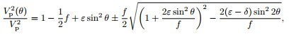
Based on the Christoffel equation and the Thomsen’s weak anisotropy theory, we can obtain the P-SV wave phase velocity dispersion equation for VTI media (Tsvankin, 1996; Alkhalifah, 1998, 2000):
|
(1) |
where 
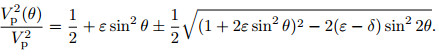
Following Alkhalifah’s TI acoustic approximation theory (assuming the shear wave velocity equals to zero directly) (Alkhalifah, 1998), we can derive the frequency-space domain qP wave equation for 2D VTI media.
Setting the shear wave velocity VSz=0, then f=1, substituting it into formula (1) yields
|
(2) |
By operating some algebraic transformation towards the formula (2) and utilizing 

|
(3) |
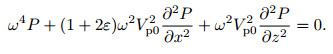
By transforming formula (3) from the wavenumber domain to the space domain, we derive the frequency-space domain qP wave equation for 2D VTI media:

|
(4) |
where P is the seismic wavefield, ω is the angular frequency, and Vp0 is the qP wave velocity for VTI media.
When ε=δ, formula (4) is simplified into frequency-space domain qP wave equation for 2D elliptic anisotropic media:
|
(5) |
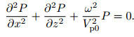
Furthermore, when ε=δ=0, formula (4) is simplified into frequency-space domain qP wave equation for 2D isotropic media.
|
(6) |
Therefore, the frequency-space domain qP wave equation for 2D elliptic anisotropic media and 2D isotropic media can be regarded as a special case of the frequency-space domain qP wave equation for 2D VTI media.
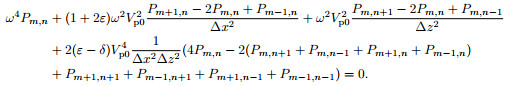
3 2D VTI Media Frequency-Space Domain qP Wave Equation 9-Point Scheme Based on ADMThe frequency-space domain qP wave equation for 2D VTI media (formula (4)) can be represented as the form of conventional 9-point scheme for 2D VTI media (Fig. 1a):

|
Fig. 1 (a) VTI conventional 9-point scheme; (b) VTI ADM 9-point scheme |
|
(7) |
The conventional 9-point scheme for 2D VTI media has a poor computational accuracy (Fig. 2). Therefore, we need to develop a new optimization algorithm. Based on the idea of ADM to construct frequency-space domain finite difference scheme for scalar wave equation (Chen, 2012; Zhang et al., 2014), we construct a new ADM 9-point scheme for 2D VTI media (Fig. 1b).

|
Fig. 2 Phase velocity curves of the VTI conventional 9-point scheme and the VTI ADM 9-point scheme for different  |
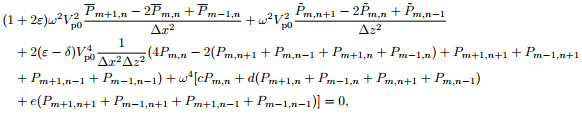
For formula (4), we represent the second-order centered spatial-derivative term and the acceleration term as a form of weighted average. Specifically, we represent the second-order finite-difference approximations of the second-order centered spatial-derivative terms as the weighted average of 3 grid points in orthogonal directions and the acceleration term ω4P as the weighted average of all 9 grid points. We introduce ADM idea into the second-order centered spatial-derivative term 


|
(8) |
where
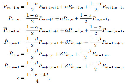
|
where α, β, c, d are weighted optimized coefficients. When α=β =1, c=1, d=0, the VTI media ADM 9-point scheme can be written as the VTI media conventional 9-point scheme. Therefore, the VTI media conventional 9-point scheme can be regarded as a special case of the VTI media ADM 9-point scheme. We increase the computational accuracy and reduce the numerical dispersion of VTI media FDFDM by introducing the ADM optimal method (Fig. 2).
4 OPTIMIZED COEFFICIENT CALCULATION AND DISPERSION ANALYSISWe perform numerical dispersion analysis on this new scheme by adopting a classic plane wave numerical dispersion analysis method.
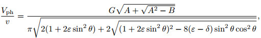
We firstly consider the condition of ∆x≥∆z for the numerical dispersion analysis. Setting 
|
(9) |
where
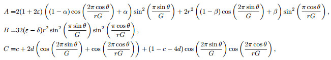
|
where G is the grid points per wavelength. Setting α=β=1, c=1, d=0, we can obtain the phase velocity dispersion formula of the VTI media conventional 9-point scheme:
|
(10) |
where

|
The optimized coefficients α, β, c, d can be determined by solving the minimum of misfit function E(α, β, c, d):
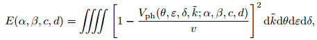
|
(11) |
where 
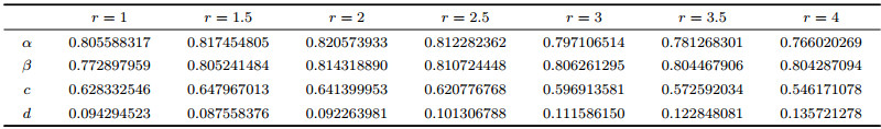
We use the least-square optimal method to calculate the optimized coefficients of the VTI media ADM 9-point scheme. The solved optimized coefficients for different 
|
|
Table 1 Optimized coefficients for different |
Considering the geometrical symmetry of the VTI media ADM 9-point scheme in two cases of ∆x≥∆z and ∆x < ∆z, as for the case of ∆x < ∆z, the only change is that the optimized coefficients corresponding to ∆x and ∆z are exchanged (Chen, 2012, 2014). The solved optimized coefficients for different 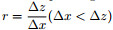
|
|
Table 2 Optimized coefficients for different  |
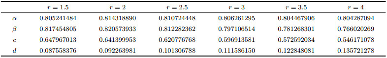
Figure 2 displays the phase velocity dispersion curves of the VTI media ADM 9-point scheme and the VTI media conventional 9-point scheme respectively for different 
Combined with the frequency-space domain PML absorbing boundary condition (Berenger, 1994; Wu et al., 2007; Zhang et al., 2014; Moreira et al., 2014), we construct the 2D VTI media ADM 9-point frequency-space domain with the PML wave equation (Appendix A). We can perform the VTI media ADM 9-point frequencyspace domain modeling by combining the optimized coefficients of different ratio of the horizontal sampling interval and the vertical sampling interval with the VTI media ADM 9-point PML wave equation. We use a complex BP2007 2D VTI ocean standard model to verify the validity and precision of the VTI media ADM 9-point scheme. As the VTI media conventional 9-point scheme is also suitable for unequal directional sampling intervals, we decide to take this scheme for comparison.
We consider a complex BP2007 2D VTI ocean standard model. Fig. 3 shows part of this model. This truncated model includes a high-velocity isotropic salt dome surrounded by VTI media and the marine layer is isotropic. The VTI media parameters include P-wave velocity VP, Thomsen anisotropic parameters ε and δ (Fig. 3). The numbers of horizontal and vertical samplings are Nx=401 and Nz=361, respectively. The horizontal sampling interval and the vertical sampling interval are 10 m and 4 m, respectively, so the ratio of the horizontal sampling interval to the vertical sampling interval comes to 2.5, the optimized coefficients of this ratio are shown in Table 1.

|
Fig. 3 Parameters of truncated BP2007 2D VTI ocean standard model (a) Vp; (b) ε; (c) δ. |
A Ricker wavelet with peak frequency of 15 Hz is placed at (x=3000 m, z=40 m) as a source. The receivers are placed at 40 m (cable sinking depth) beneath the sea surface with a spacing of 10 m. We adopt the frequencyspace domain PML absorbing boundary condition and the PML thickness is 40 layers. The propagation time is 2 s and the time sampling interval is 4 ms.
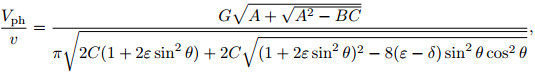
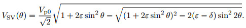
It is worth noted that VTI media frequency-space domain qP wavefield propagation process often appears with strong pseudo-shear wave (pseudo-SV wave) noise by practical tests. The pseudo-SV wave noise is caused due to the TI acoustic approximation (Grechka et al., 2004). By referencing the following SV wave phase velocity formula (12) presented by Grechka, we can easily conclude that the TI acoustic approximation only makes the shear velocity in the direction of symmetrical axis be zero, whereas the shear velocity in the other propagation direction is not zero which causes strong pseudo-SV wave noise. This kind of pseudo-SV wave noise must be suppressed and eliminated, because it will cause serious interference in practical migration and inversion and may lead to instability of the algorithm though this pseudo-SV wave noise reflects the characteristics of low velocity and low energy compared with qP wave. Through analysis we conclude that the pseudo-SV wave noise can be eliminated effectively by adding an elliptic anisotropic layer or an isotropic thin layer around the source. So the strategy of adding an isotropic thin layer around the source can eliminate pseudo-SV wave noise effectively during the VTI media qP wavefield propagation.
|
(12) |
However for our example, the source is placed in the isotropic marine layer. The pseudo-SV wave noise will not appear during the VTI media qP wavefield propagation. Therefore we don’t need to consider the strategy of adding an isotropic thin layer around the source to eliminate pseudo-SV wave noise for this case.
We perform frequency-space domain forward modeling by using VTI media conventional 9-point scheme and the VTI media ADM 9-point scheme respectively. Fig. 4a is the 35 Hz monochromatic wavefield computed by the VTI media ADM 9-point scheme. We can see that the frequency-space domain wavefield characteristic of qP wave is very clear and depicts well. The frequency-space domain wavefield changes slowly in the right part of the model because the velocity and anisotropic parameters varies gradually. But the frequency-space domain wavefield around the steep salt dome disturbs abruptly because the velocity and anisotropic parameters vary complicatedly. The incident wave and reflected wave interference to each other on the reflecting interface.

|
Fig. 4 (a) 35 Hz monochromatic wavefield computed by VTI ADM 9-point scheme; (b) Time-domain seismograms computed with the VTI conventional 9-point scheme; (c) Time-domain seismograms computed with the VTI ADM 9-point scheme; (d) Time-domain seismograms computed with the time domain 12-order high order finite difference scheme for VTI media |
We can get the time-domain seismograms by using inverse fast Fourier transform towards frequency-space domain wavefield of all frequencies. Time-domain seismograms computed with the VTI media conventional 9-point scheme and the VTI media ADM 9-point scheme are shown in Figs. 4b and 4c, respectively. From the figures, we can see that the result of the VTI media ADM 9-point scheme is much better than that of the VTI media conventional 9-point scheme. The simulation result with the VTI media ADM 9-point scheme is more accurate while the result with VTI media conventional 9-point scheme exhibits errors due to numerical dispersion. More specifically, the maximum frequency is about 40 Hz and the minimum velocity is 1492 m·s−1 (Sea-water velocity). Therefore according to the dispersion criterion, the VTI media conventional 9-point scheme needs dx=1492/40/12=3.1 m to avoid numerical dispersion whereas the VTI media ADM 9-point scheme only needs dx=1492/40/3.57=10.4 m. For this example, horizontal sampling interval (10 m) obviously exceeds the allowed sampling interval of the VTI media conventional 9-point scheme for accurate modeling (3.1 m). So the VTI media conventional 9-point scheme causes serious numerical dispersion but the VTI media ADM 9-point scheme can simulate accurately.
Figures 4b and 4c also show that the frequency-space domain PML absorbing boundary condition eliminates the artificial boundary reflection very well. The simulation results also demonstrate the VTI media ADM 9-point scheme is in good agreement with the high-precision time domain 12-order high order finite difference scheme for VTI media (Duveneck and Bakker, 2011) (Fig. 4d).
We perform a computational efficiency test in the same computational domain and the same computational accuracy on the BP2007 2D VTI ocean standard model (the same computational accuracy means just do not produce numerical dispersion). The computing platform is ThinkCentre M8500t desktop PC (Core i7 eightcore). The simulation result is that the computation time of the VTI media conventional 9-point scheme is 10262 s whereas that of the VTI media ADM 9-point scheme is only 2730 s. Therefore the computational efficiency of the VTI media ADM 9-point scheme is significantly higher than the VTI media conventional 9-point scheme. This is because the VTI media ADM 9-point scheme can significantly increase the computational accuracy compared with the VTI media conventional 9-point scheme, so the new scheme can use a larger grid interval to improve the computational efficiency.
In terms of memory storage, if the VTI media conventional 9-point scheme needs Nx × Nz (Nx and Nz are horizontal and vertical samplings respectively) grid points to storage coefficient matrix, then the new scheme only needs 
The VTI media conventional 9-point scheme can cause serious numerical dispersion because of its poor computational accuracy. In this paper, we propose a new kind of VTI media ADM 9-point scheme which significantly increases the computational accuracy of VTI media FDFDM compared with the VTI media conventional 9-point scheme. We obtain the optimized coefficients by using the least-square optimal method to minimize numerical dispersion and decrease the required grid points per wavelength to 3.57 bounded by a phase velocity error range of±1%, whereas the VTI conventional 9-point scheme needs approximately 12 grid points per wavelength bounded by the same error range. Therefore the new scheme possesses advantage in terms of overcoming numerical dispersion. The numerical example demonstrates that the VTI media ADM 9-point scheme can not only possess high computational precision and computational efficiency, but also possess applicability and flexibility. The VTI media ADM 9-point scheme can be developed further and has many applications. Taking FWI for example, VTI media ADM 9-point scheme can be applied to the VTI FWI as a fast and accurate modeling engine.
Appendix A Constructing the 2D VTI Media ADM 9-Point Frequency-Space Domain PML Wave EquationBy introducing the PML technique (Berenger, 1994; Moreira et al., 2014), we combine the 2D PML stretch function ex and ez in the frequency-space domain with the frequency-space domain qP wave equation for 2D VTI media (formula (4)) and derive the frequency-space domain qP wave equation for 2D VTI media with the PML absorbing boundary condition:
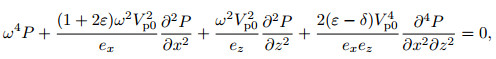
|
(A1) |
where
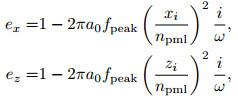
|
where fpeak is the peak frequency of a Ricker wavelet, xi and zi are the distance from the inner boundary point to the inner edges of the PML layers, and npml is the width of the PML layer. The coefficient a0 is an empirical value which is 1.79 in this paper (Wu et al., 2007).
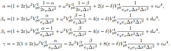
We combine the formula (A1) with the 2D VTI media ADM 9-point scheme (formula (8)) and derive the ADM 9-point finite difference scheme for 2D VTI media with the PML absorbing boundary condition:

|
(A2) |
where
|
The seismic wavefield will attenuate gradually when wave propagates from the internal computational domain to the PML boundary layer.
ACKNOWLEDGMENTSWe thank the two anonymous reviewers for their comments and suggestions and the editor’s careful and responsible work in improving the manuscript. This research was supported by the National Science and Technology of Major Projects (2011ZX05003-003), the National Natural Science Foundation of China (NSFC) (41176056) and the National 863 Program of China (2012AA061202).
| [] | Alkhalifah T. 1998. Acoustic approximations for processing in transversely isotropic media. Geophysics , 63 (2) : 623-631. DOI:10.1190/1.1444361 |
| [] | Alkhalifah T. 2000. An acoustic wave equation for anisotropic media. Geophysics , 65 (4) : 1239-1250. DOI:10.1190/1.1444815 |
| [] | Alkhalifah T. 2014. Full Waveform Inversion in an Anisotropic World:Where are the Parameters Hiding? Houten, The Netherlands:EAGE Publications bv. |
| [] | Berenger J P. 1994. A perfectly matched layer for the absorption of electromagnetic waves. Journal of Computational Physics , 114 (2) : 185-200. DOI:10.1006/jcph.1994.1159 |
| [] | Chen J B. 2012. An average-derivative optimal scheme for frequency-domain scalar wave equation. Geophysics , 77 (6) : T201-T210. DOI:10.1190/GEO2011-0389.1 |
| [] | Chen J B. 2014. Dispersion analysis of an average-derivative optimal scheme for Laplace-domain scalar wave equation. Geophysics , 79 (2) : T37-T42. DOI:10.1190/GEO2013-0230.1 |
| [] | Cheng J B, Kang W, Wang T F. 2013. Description of qP-wave propagation in anisotropic media, Part 1:Pseudo-puremode wave equations. Chinese J. Geophys. (in Chinese) , 56 (10) : 3474-3486. DOI:10.6038/cjg20131022 |
| [] | Du X D, Liu J R, Qi Y P, et al. 2009. Finite difference high-order weighted-averaging operator for frequency-space domain qP wave in 3-D VTI media. Progress in Geophys. (in Chinese) , 24 (1) : 211-222. |
| [] | Duveneck E, Bakker P M. 2011. Stable P-wave modeling for reverse-time migration in tilted TI media. Geophysics , 76 (2) : S65-S75. DOI:10.1190/1.3533964 |
| [] | Grechka V, Zhang L B, Rector J W. 2004. Shear waves in acoustic anisotropic media. Geophysics , 69 (2) : 576-582. DOI:10.1190/1.1707077 |
| [] | Grini M, Ribodetti A, Virieux J, et al. 2007. Finite-difference frequency-domain modeling of acoustic wave propagation in 2D TTI anisotropic media.//69th Annual EAGE Conference and Exhibition, EAGE Extended Abstracts, 323. |
| [] | Li G H, Feng J G, Zhu G M. 2011. Quasi-P wave forward modeling in viscoelastic VTI media in frequency-space domain. Chinese J. Geophys. (in Chinese) , 54 (1) : 200-207. DOI:10.3969/j.issn.0001-5733.2011.01.021 |
| [] | Lines L R, Treitel S. 1984. A review of least-squares inversion and its application to geophysical problems. Geophysical Prospecting , 32 (2) : 159-186. DOI:10.1111/j.1365-2478.1984.tb00726.x |
| [] | Min D J, Shin C, Kwon B D, et al. 2000. Improved frequency-domain elastic wave modeling using weighted-averaging difference operators. Geophysics , 65 (3) : 884-895. DOI:10.1190/1.1444785 |
| [] | Moreira R M, Santos M A, Martins J L, et al. 2014. Frequency-domain acoustic-wave modeling with hybrid absorbing boundary conditions. Geophysics , 79 (5) : A39-A44. DOI:10.1190/GEO2014-0085.1 |
| [] | Operto S, Ribodetti A, Grini M, et al. 2007. Mixed-grid finite-difference frequency-domain viscoacoustic modeling in 2D TTI anisotropic media.//77th Annual International Meeting, SEG Expanded Abstracts, 2099-2103. |
| [] | Operto S, Virieux J, Ribodetti A, et al. 2009. Finite-difference frequency-domain modeling of viscoacoustic wave propagation in 2D tilted transversely isotropic (TTI) media. Geophysics , 74 (5) : T75-T95. DOI:10.1190/1.3157243 |
| [] | Operto S, Brossier R, Combe L, et al. 2014. Computationally efficient three-dimensional acoustic finite-difference frequency-domain seismic modeling in vertical transversely isotropic media with sparse direct solver. Geophysics , 79 (5) : T257-T275. DOI:10.1190/GEO2013-0478.1 |
| [] | Shin C S, Sohn H J. 1998. A frequency-space 2-D scalar wave extrapolator using extended 25-point finite-difference operator. Geophysics , 63 (1) : 289-296. DOI:10.1190/1.1444323 |
| [] | Thomsen L. 1986. Weak elastic anisotropy. Geophysics , 51 (10) : 1954-1966. DOI:10.1190/1.1442051 |
| [] | Tsvankin I. 1996. P-wave signatures and notation for transversely isotropic media:An overview. Geophysics , 61 (2) : 467-483. DOI:10.1190/1.1443974 |
| [] | Tsvankin I. 2001. Seismic Signatures and Analysis of Reflection Data in Anisotropic Media. United Kingdom:Elsevier Science. |
| [] | Tsvankin I, Gaiser J, Grechka V, et al. 2010. Seismic anisotropy in exploration and reservoir characterization:An overview. Geophysics , 75 (5) : 75A15-75A29. DOI:10.1190/1.3481775 |
| [] | Warner M, Ratclife A, Nangoo T, et al. 2013. Anisotropic 3D full-waveform inversion. Geophysics , 78 (2) : R59-R80. DOI:10.1190/GEO2012-0338.1 |
| [] | Wu G C, Liang K. 2005. Quasi P-wave forward modeling in frequency-space domain in VTI media. Oil Geophysical Prospecting (in Chinese) , 40 (5) : 535-545. |
| [] | Wu G C. 2006. Seismic Wave Propagation and Imaging in Anisotropic Media (in Chinese)[M]. Dongying: China University of Petroleum Press . |
| [] | Wu G C, Luo C M, Liang K. 2007. Frequency-space domain finite difference numerical simulation of elastic wave in TTI media. Journal of Jilin University (Earth Science Edition) (in Chinese) , 37 (5) : 1023-1033. |
| [] | Wu G C, Liang K. 2007. High precision finite difference operators for qP wave equation in VTI media. Progress in Geophys. (in Chinese) , 22 (3) : 896-904. |
| [] | Zhang H, Liu H, Liu L, et al. 2014. Frequency domain acoustic equation high-order modeling based on an averagederivative method. Chinese J. Geophys. (in Chinese) , 57 (5) : 1599-1611. DOI:10.6038/cjg20140523 |
| [] | Zhang Y, Wu G C. 2013. Review of prestack reverse-time migration in TTI media. Progress in Geophys. (in Chinese) , 28 (1) : 409-420. DOI:10.6038/pg20130146 |