 2015, Vol. 58


2 Institute of Geology and Geophysics, Chinese Academy of Sciences, Beijing 100029, China
Earthquake location plays a fundamental role in seismic researches on seismicity, nuclear test monitoring and Earth’s interior structure (Zeng, 1991; Ding et al., 1999; Richards et al., 2006; Chen, 2009). To accurately determine sources’ positions and origin times, seismologists have developed various location methods (Tian et al., 2002; Cai et al., 2004; Yang et al., 2005), such as the Geiger method (Geiger, 1912), the double-difference algorithm (Waldhauser et al., 2000), the grid-search scheme (Shearer, 1997), the intersection method (Pujol, 2004; Lian et al., 2006; Zhou et al., 2012) and the time-reversal imaging technique (Xu et al., 2013a and 2013b). These location methods have their own characteristics. Compared with others, the intersection location method has advantages including excellent simplicity, visuality and robustness, and thereby is widely used in seismic networks (Meng et al., 2001; Song et al., 2001). Its basic idea is to determine the hypocenter using hypocentral loci. As a result, valuable information on the hypocenter can be obtained even when there is a few of seismic records available for use (Zhao et al., 2008). On the other hand, the intersection method is deficient in location accuracy, especially for focal depth (UdÍas, 1999). This is mainly attributed to the fact that the reference model is assumed to be homogeneous or laterally homogeneous (the focal loci in these cases have analytical solutions). In the real earth, however, there are large lateral as well as radial velocity variations. The discrepancy between the reference model and the real Earth inevitably results in different degrees of source bias (Billings et al., 1994; Chen et al., 2006). So, modifying the intersection method to be suitable to complex velocity models is critical for improving its location accuracy. Besides, highly accurate location based on 3-D models has become a reachable target because more and more regional three dimensional velocity models are constructed with considerable accuracy and the resolution of global structure image is continually improved, which greatly benefits from the development of seismic networks and inversion techniques.
Expansion of the conventional intersection method to a three dimensional velocity model firstly involves the calculation of hypocentral loci, which can rarely be expressed analytically when the velocity varies in three dimensions. As for the problem of calculating focal loci in complex media, there are presently two main schemes. One is representing a hypocentral locus with the points that satisfy the locus equation within a prescribed tolerance (Zhou, 1994; Font et al., 2004; Theunissen et al., 2012). This scheme is straightforward and adaptive, and hence has no restrictions on the geometry of hypocentral loci. However, resultant rough loci do not intersect at one point but to form a region even when the velocity model and picked arrival times are both accurate, especially for a large tolerance. The other one is based on a minimum travel time algorithm for tracing rays: A hypocentral locus is represented by the ray paths from the minimal point (namely the initial point) to low valued points (referred as hypocentral locus reference points, HLRPs) in its residual field (Zhao et al., 2008). The ray-tracing based scheme can produce such fine hypocentral loci that their directional distribution allows us to directly estimate the location quality and visually analyze the effects of the velocity model, the observed arrivaltime and the station distribution on the location result. Its major disadvantages are that (1) it can not correctly deal with multi-segmented loci: When a hypocentral locus consists of two or more separate segments, the scheme will produce false locus, namely, the rays connecting individual locus segments because only the minimal point in the residual filed is set as the initial point which is connected to all the HLRPs by rays; (2) it does not satisfy the requirement of processing large batches of data because the selection of HLRPs is rather laborious: HLRPs are chosen at a percentage of the number of all model nodes, and the percentage is required to vary with the length of hypocentral locus while the locus length can hardly be known in advance; (3) it is poorly adapted for producing both fine and complete loci: Even though the locus length is known, HLRPs selected purely according to the residual value are either so insufficient that they do not characterize the locus completely or so excessive that the resultant locus is rough because the residual differs at the nodes of the elements that a hypocentral locus goes through. Actually, earthquakes recorded by and observed data from modern seismic networks are both very large in quantity. For accurately locating large numbers of seismic events, hypocentral loci are required to be calculated with high efficiency and accuracy.
Thus it is clear that the solution for calculating hypocentral loci in complex media needs to be improved further. In this study, we attempt to modify the calculation method based on a ray tracing algorithm (Zhao et al., 2008) to overcome its disadvantages. For convenience, the methodology is illustrated using a 2D model.
2 EQUATIONS OF HYPOCENTRAL LOCIPresume that the velocity model of a region is known and on the ground there are M seismic stations, Ri(i=1, 2, 3, …, M). To locate earthquakes within the region, we divide the region’s velocity model into equal square elements. Within an element, the seismic velocity is constant and the central point of the cell is a node of the model. We employ a minimum traveltime tree algorithm for tracing rays (Zhao et al., 2003, 2004) to calculate travel times of the first-break primary (P) and shear (S) waves from a station Ri(i=1, 2, 3, …, M) (the shot points are placed at stations) to each node with coordinates x=(x, z) of the region, T (x; Ri, P) and T (x; Ri, S)(i=1, 2, 3, …, M). As for the earthquake with the hypocenter at x0=(x0, z0) and the origin time of t0 in the region, the P-and S-wave first arrivals from the hypocenter to the seismic station Ri are denoted by τRiP and τRiS respectively. According to the hypocenter-station symmetry, we can construct two kinds of equations of hypocentral loci constrained with arrival time differences and arrival times, respectively.
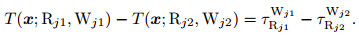
2.1 Hypocentral Loci Constrained with Arrival Time DifferencesEvery two observed arrival times constitute one arrival time pair. For the jth arrival time pair, its two components are respectively denoted by τRj1Wj1 and τRj2Wj2, where Rj1 and Rj2 represent the seismic stations recording the two arrival times; Wj1 and Wj2 are the types of seismic phases, i.e., P or S. The hypocentral locus constrained with the difference between τRj1Wj1 and τRj2Wj2 meets the following equation (Zhao et al., 2008):
|
(1) |
The equation above indicates that the focal locus is of quite small values near zero, taking calculation errors into account, in the following residual field with respect to travel time difference:

|
(2) |
where I(x)=1.
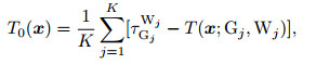
2.2 Hypocentral Loci Constrained with Arrival TimesUsing the observed arrival times, we can construct an origin time field of the event as follows (Zhao, 2014):
|
(3) |
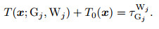
where Gj and Wj are respectively the station and the seismic phase type (P or S wave) of the jth arrival time, and K is the number of the arrival times observed. Hence, the hypocentral locus constrained with the jth arrival time meets the following equation:
|
(4) |
The Eq.(4) indicates that the focal locus is of quite small values near zero, taking calculation errors into account, in the following residual field with respect to arrival time:

|
(5) |
where I(x)=1.
Equations (1) and (4) have exact analytical solutions only when the velocity model is very simple. Different from hypocentral loci constrained with arrival time differences, the ones constrained by arrival times are rather complex even for homogeneous media, especially when the origin time field is constructed using many arrival times. Let us consider a homogeneous model with the dimensions of 150 km×90 km. The P-and S-wave velocities are 6.0 km·s−1 and 3.6 km·s−1, respectively. We divide the model into square cells of 3 km×3 km. Assume that an earthquake is triggered at x0(37.5 km, –31.5 km) and t0=0 s. The P-and S-waves from the event are recorded by five stations, Ri(13.5 + (i − 1) × 30.0 km, –1.5 km) (i=1, 2, 3, …, 5). Fig. 1 shows the origin time fields of the event and the arrival time residual fields corresponding to the P-wave arrival at the station R3. The grey scale of Fig. 1c and 1d is proportional to the residual value. In order to clearly show the focal loci, the residual values have been normalized and converted into base-10 logarithms. From Fig. 1, it can be seen that 1) the origin time field constructed with only P-wave arrivals (Fig. 1a) is similar in structure to that with both P-and S-wave data (Fig. 1b), which results from the constant velocity ratio of the two modes of waves; 2) the hypocentral locus constrained with only P waves (Fig. 1c) and that with both P-and S-waves (Fig. 1d) are not circular or hyperbolic, but much more complex, especially the latter consists of two separate segments; 3) for different origin time fields, hypocentral loci constrained with the same arrival time are not same, even are entirely different.

|
Fig. 1 Origin time fields (a, b) and arrival time residual fields (c, d) of an event in a homogeneous medium (a) P-wave arrival times; (b) P-and S-wave data; (c) and (d) one P-wave arrival time jointed with the origin time fields (a) and (b), respectively. The origin time contour interval equals 2.0 s, and the red crosses indicate the hypocenter. In the residual fields, the green lines are contours of 0.2 s. The blue solid and red dashed lines respectively show the calculated and theoretical focal loci. The yellow dots indicate the selected hypocentral locus reference points. |
In a residual field described by Eq.(2) or (5), points on the hypocentral locus bear extremely small values, as Fig. 1 shows. The low residual (e.g., smaller than 0.2 s) area is divided in accordance with the geometry of the hypocentral locus into one (Fig. 1c) or more (Fig. 1d) connected regions. Assume that sources are exploded simultaneously at the minimum points in these separate connected regions. The seismic waves certainly will travel fast along the focal locus, but spread slowly in areas beyond it, especially outside the connected regions, where the field value is regarded as that of seismic slowness. We characterize the hypocentral locus using some nodes (referred as the reference points of the hypocentral locus, HLRPs), and assign the point with minimal residual of every connected region as an initial point. In this way, ray paths from the initial points to their respective HLRPs that lie in the same connected regions with themselves approximately represent the hypocentral locus, and there are no false hypocentral loci. For the convenience of treatment, nodes with residual below a given threshold are usually assigned as hypocentral locus reference points (Zhou, 1994; Zhao et al., 2008). As is illustrated by different gray scales in Figs. 1c and 1d, the residual varies considerably at the nodes of the cells that the hypocentral locus runs through. Therefore, it is rather difficult to obtain both fine and complete loci. When nodes of the cells crossed by the hypocentral locus are chosen as the HLRPs, the resultant hypocentral locus is quite fine and complete. Based on this analysis, we propose an improved method for calculating hypocentral loci in complex media.
3.1 Selection of Reference PointsThe hypocentral locus lies in the middle of connected regions with low residuals, just like one or more cores of a fruit, as can be seen from Figs. 1c and 1d. As for nodes of the cells that the hypocentral locus goes through, their residuals are different considerably but are respectively minimal, compared with ones at their two sides beyond the locus. According to the characteristic of such nodes, we can select them in a way similar to the one that we get the core of a fruit by repeatedly cutting off its outside layer. For the sake of description, nodes with residuals below RFLRP are referred to as the primary HLRPs and their set is denoted by Θ. The scheme for selecting HLRPs from the set Θ can be expressed as follows:
(1) Classification
A node i ∈ Θ is classified as one inner point of the set Θ if its adjacent points all belong to Θ; otherwise it is classified as one outside point of the set Θ. The sets of inner and outside nodes are denoted by I and O, respectively.
(2) Updating
A node i ∈ O is retained if among its adjacent points there are no or only such inner points that they bear bigger residuals than the node i; otherwise it is removed from the set O. After this operation is done for all members of the set O, the set Θ is updated as the union of the sets O and I.
(3) Iteration check
If the set I becomes empty go to (4); otherwise go to (1).
(4) Simplification
The set O sometimes includes such members that they are distributed in two lines side by side, along the hypocentral locus. In this case, we simplify the set O, for only one of the two lines is required for characterizing the locus. As for the node i ∈ O and its adjacent outside points, when they are more than three, we retain only the three minimum-residual ones.
(5) Purification
When the residual field is complex, the set O may include a few of outliers, which lie away from the hypocentral locus. In this study, a node with the residual larger than the average of all the points in O by two standard deviations is regarded as one outlier, and removed from O.
In the algorithm above, step (1)-(3) stands for the layer-by-layer removal of the outside members of the set of primary HLRPs in a similar way of peeling a fruit. Step (4) stands for the removal of superfluous reference points and step (5) for that of false ones. The points retained finally in the set O are used as HLRPs. In Figs. 1c and 1d, the yellow points are HLRPs selected from the primary ones with residuals of less than 0.2 s. It can be seen that the selected HLRPs characterize the hypocentral locus fairly well and hence are sufficient for calculating the locus although they are just a part of nodes that the hypocentral locus goes through. Actually, for the calculation of a hypocentral locus represented by ray paths, it is preferable to choose only the minimal residual node and the two end ones of each segment of the locus as the HLRPs but is difficult to realize.
3.2 Calculation of Ray PathsRay paths representing the hypocentral locus are calculated with an improved minimum traveltime tree algorithm (Zhao et al., 2004). The minimum traveltime tree algorithm for tracing rays (Nakanishi et al., 1986; Moser, 1991) is based on Huygens’ Principle and Fermat’s Principle in Seismology, and has an advantage of excellent robustness suitable for complex velocity models. Travel times and ray paths from the shot point to all nodes in the model are calculated simultaneously by constructing a minimum traveltime tree (Cao et al., 1993). As for a hypocentral locus consisting of multiple segments, in order to prevent from producing false hypocentral locus, the minimal residual point in each connected region that contains one segment of the hypocentral locus is required to be assigned as an initial point of seismic waves. Such initial points of all the connected regions are difficult to determine at the same time because the distribution of the hypocentral locus can hardly be known in advance. On the other hand, the minimum traveltime tree algorithm runs within a connected region, which is concluded by its ending condition. So, we restrict the calculation of ray paths to a low residual area and then employ the minimum traveltime tree algorithm to calculate the hypocentral locus by assigning in turn the initial points of the connected regions. As HLRPs include the minimal residual points of all the connected regions, initial points of seismic waves can be chosen from them.
The calculation domain of ray paths is defined as the area Ω with the residual of less than RFL, which can be realized by setting the nodes outside Ω as the points at which the travel time has been minimum. In this subsection, the set of HLRPs selected from the nodes with the residual of less than RFLRP is denoted by Z. The parameters RFL and RFLRP can be set same or different. The algorithm for tracing rays representing a hypocentral locus can be described as follows:
(1) Selection of the initial point
Find the node s ∈ Z with the minimum residual and remove it from Z.
(2) Calculation of ray paths
Take s as the initial point and run the minimum traveltime tree algorithm to calculate travel times and ray paths of the seismic waves in the residual field until it stops; if a node j ∈ Z has been traced then remove it from Z.
(3) Iteration check
If Z becomes an empty set then stop; otherwise go to (1).
3.3 Modification of Hypocentral LociMost of the reference points of a hypocentral locus do not exactly but approximately satisfy the locus equation. When their amount is excessive, the calculated focal locus is probably rather crude and needs some modifying.
Ray paths from the HLRPs to their perspective initial points of seismic waves form one or more tree structures, as Fig. 2 shows. Thus, we regard the rays as tree branches (directed line segments in Fig. 2) and the nodes that they go through as branch origins. A branch origin is also one branching point when the number of branches sprouting from it (figure in the circle) is not less than two. The trunk of the ray tree (namely the part constituted by the rays from the initial point to the HLRPs that there are not less than nFLP rays going through, such as line segment BCD) certainly lies on the actual hypocentral locus. However, selecting the part only (Zhao et al., 2008) probably harms the intactness of a hypocentral locus. For example, hypocentral locus segment GHI in Fig. 2 will be lost for nFLP=2. Therefore, for the sake of the completeness and the fineness of the calculated hypocentral locus, we remove the twigs without branching and with a length less than Ltwig, such as the dashed lines in Fig. 2.

|
Fig. 2 A diagram of one hypocentral locus represented with ray paths |
The blue lines in Figs. 1c and 1d are the corresponding calculated hypocentral loci for nFLP=2 (in unit of the length of the element side). Clearly, the calculations are quite consistent with the real loci (the red dashed lines). Certainly, the consistence between them is better when the model is divided into smaller (e.g., 1 km×1 km) cells.
4 EXAMPLES OF CALCULATION 4.1 Virtual Event 4.1.1 Velocity modelThe virtual event is designed against a background of Yunnan area, China. Yunnan area is characterized by active seismicity, and its deep structure has been investigated by many geophysical explorations (Kan et al., 1986; Wang et al., 2002). As a result, there are a number of high-resolution velocity profiles constructed from the deep seismic sounding data (Bai and Wang, 2003; Zhang et al., 2011; Teng et al., 2013). We slightly smoothed the Zhefang-Binchuan velocity profile (Bai and Wang, 2003) and obtained a model as shown by Fig. 3. The P-wave to S-wave velocity ratio vS : vP is taken as a constant 1:1.73. It is clear that the model is strongly heterogeneous in lateral and vertical directions. We divide the model into 1 km×1 km elements and set the velocity constant within an element. In the top surface, there are 9 stations Ri(i=1, 2, 3, …, 9), whose positions are listed in Table 1. Assume that an earthquake occurs at x0(130.5 km, –27.5 km) with the origin time t0=0 s. Traveltimes and ray paths of the P-and S-waves from the hypocenter to the stations are calculated with an improved minimum traveltime tree algorithm (Zhao et al., 2004). The ray paths are shown as the black lines in Fig. 3.
|
|
Table 1 Positions of the seismic receivers in the complex model |


|
Fig. 3 A complex model (from Bai et al., 2004) The black lines are ray paths of seismic waves from the hypocenter (cross) to stations (inverse triangles). |
As for the earthquake in Fig. 3, we apply the modified method to calculate its two kinds of hypocentral loci, which are constrained with arrival times and arrival time differences, respectively. Arrival time difference constrained hypocentral loci each involve only two arrivals and hence are fairly independent. They have also been studied in detail (Bai et al., 2003; Lian et al., 2006; Zhao et al., 2007, 2008, 2009; Theunissen et al., 2012). Contrastingly, arrival time constrained ones are not only dependent upon their respective arrival times but also related to those constructing their origin time fields. Furthermore, they are poorly researched. Therefore, as for the former, we calculate them in only the case of all stations, a correct velocity model and precise arrival times; whereas, as for the latter, we investigate them in different observation cases (for example, all stations, sparse stations, near stations, far stations and one-side stations) when the velocity model and the arrival times are all correct and in the case that all the stations are employed, the velocity model is accurate but the arrival times are randomly perturbed. All the hypocentral loci are calculated with a set of parameters: RFLRP=0.1 s, RFL=0.2 s, Ltwig=5.
4.1.2 Hypocentral loci constrained with arrival time differencesIn theory, P-wave arrivals at the 9 stations can be pairwise combined into C92=36 arrival time differences. Among the hypocentral loci constrained with these differences, some ones are much alike in directional distribution. Herein we select ten representative hypocentral loci as shown in Fig. 4a. The character pair “i − j” beside a locus signifies that the locus is constrained with the arrival time difference τRjP − τRjP and the signal of red “+” represents the real hypocenter. One can see that the resultant hypocentral loci are all fine and quite complete without adjusting the calculation parameters; their directional distribution is fairly isotropic and complete near the hypocenter and results in a tight constraint upon the hypocenter; as for station twins symmetrical with respect to the epicenter, the arrival time difference constrained hypocentral loci (i.e. locus “1–9”) trend in nearly vertical directions near the hypocenter, and tightly constrain the epicenter while as for those away from the epicenter, the corresponding ones (i.e. locus “1–3”) have strong horizontal components near the hypocenter, and appear well capable of constraining the hypocentral depth. The perfect intersection of hypocentral loci at the hypocenter results from the correctness of the velocity model and the arrival times.

|
Fig. 4 Hypocentral loci constrained with arrival time differences for the event in the complex model (a) Focal loci constrained with arrival time differences between P waves at different stations; (b) Those with ones between P and S waves at the same stations. |
Hypocentral loci constrained with arrival time differences between P and S waves at the same stations are shown in Fig. 4b. The character “i” beside a locus expresses that the locus is constrained with arrival time difference τRiS − τRIP. Obviously, the loci corresponding to stations R2 and R7 respectively consist of two separate segments, and both have been correctly calculated without producing false loci even though the velocity model is fairly complex. Similar to the hypocentral loci constrained with arrival time differences between P waves at different stations, those constrained by P and S wave differences at the same stations also have a complete directional distribution and sufficiently constrain the hypocentral location, but different from the former, their near-station loci tightly constrain the hypocentral depth and their far-station ones firmly constrain the epicenter.
When the observation is not complete, for example, only stations R5~R9 are employed, neither of the two types of hypocentral loci adequately constrains the hypocenter because of the loss of many distribution directions. On the other hand, they are strongly complementary in directional distribution and thus combining them can significantly reduce the effect of incomplete observation. When the arrival times and/or the velocity model are not accurate, it can be concluded that the resultant hypocentral loci will not cross exactly at the hypocenter but intersect into an area (See Zhao et al., 2008).
4.1.3 Hypocentral loci constrained with arrival timesHypocentral loci constrained with arrival times of P waves at all the stations are shown in Fig. 5a. Their directional distribution near the hypocenter is not as complete and isotropic as that of ones constrained with arrival time differences (Fig. 4a). They mainly have strong vertical components near the hypocenter but there are two going through the hypocenter at large angles from the vertical direction. As a result, they also sufficiently constrain the hypocentral location. When the origin time field is constructed with both P-and S-wave arrivals, the arrival time constrained hypocentral loci are shown in Fig. 5b. The blue and the green lines correspond to the P-and S-waves, respectively. As can be seen, the additional use of S-wave data resulted in a slightly improved azimuthal distribution, which is much similar to the previous one. But then it is beneficial to decreasing the influence of random noise because more hypocentral loci are available to constrain the hypocenter.

|
Fig. 5 Hypocentral loci constrained with arrival times for the event in the complex model (a) and (b) all stations; (c) and (d) sparse stations; (e) and (f) near stations; (g) and (h) far stations; (i) and (j) right-side stations; (k) and (l) noisy arrival times. Focal loci in the left panels are constrained with only P-wave arrival times; those in the right ones with both P-and S-wave data, where the blue and green lines respond to P and S waves, respectively. The red “+” indicate the true hypocenter. |
In the case of all stations, the station interval is 30 or 20 km, whereas in practice it is two or more times longer than this distance. Hence we reserve only odd stations R2i−1(i=1, 2, 3, …, 5). Fig. 5c and 5d show the hypocentral loci constrained with alone P-wave arrivals and with both P-and S-wave ones at these sparse stations, respectively. As one can see, the hypocentral loci resulting from the sparse observation have a somewhat narrower azimuthal distribution near the source, but still sufficiently constrain the hypocenter position. Similarly, there are hypocentral loci constrained with the arrival times at near stations (R2~R6), which are shown in Fig. 5e and 5f. When there are only far stations (R1, R2, R7, R8 and R9), the arrival time constrained hypocentral loci for P-waves and for both P-and S-waves trend in nearly vertical directions near the hypocenter; thereby they can hardly constrain the depth of the focus.
In the practice of location, events often take place outside the seismic network. To simulate this situation, we keep only five stations R5~R9 at the right side of the epicenter. Hypocentral loci constrained with the P-wave arrival times are shown in Fig. 5i. Notably, they trend mainly in the horizontal direction, and appear capable of tightly constraining the hypocentral depth. When the S-wave data are additionally used, the directional distribution near the hypocenter becomes sharply different from those in the previous cases. It is both quite complete and isotropic, as Fig. 5j shows. This implies that the joint use of P-and S-wave arrival times is especially important for the earthquake location under the condition of partial observation. In Fig. 5j, it also can be seen that not only all the hypocentral loci intersect exactly at the hypocenter but also partial ones intersect in the area up and right of the hypocenter. From this we conclude that the function of total arrival time residual has local minimum points. Accordingly, when an earthquake is located using the Geiger method (its objective function is total arrival time residual), the input initial values of hypocentral parameters are required to be close to the real ones.
Arrival times always include more or less errors for they are affected by various factors such as environment, instruments and operators. To investigate the effect of arrival time picking errors on the distribution of hypocentral loci, the theoretical arrival times at all the nine stations are added random perturbations within the range of±0.5 s. The perturbations are generated by a random function of FORTRAN 90 compiler. The arrival time standard deviation is 0.356 s for P waves and 0.321 s for S waves. The resultant hypocentral loci constrained with alone P-arrivals and with both P-and S-arrivals are shown in Fig. 5(k, l). Clearly, they do not cross at the hypocenter but intersect into a small area. Compared with Fig. 5k, the point where the hypocentral loci intersect most densely in Fig. 5l is nearer to the real hypocenter.
4.2 Real Event 4.2.1 Event and velocity modelThe real event comes from North China, a significant seismic monitoring area covered with a dense and nearly uniform seismic network. Since hypocentral loci are shown in a two-dimensional profile, an earthquake is desirable when its epicenter is located in a line through several stations. In the east of North China, there is an event of ML4.2 basically meeting the requirement, which occurred on August 26, 2012 (Beijing time). Reported by Beijing Digital Telemetry Seismic Network (abbreviated to BJSN), the event is at 39.61◦N, 117.42◦E, and 13 km deep; its origin time is 7 h 13 m 34.3 s. Fig. 6 shows the epicentral location and its surrounding stations. It is worth to point out that there are more stations within a bigger area. Obviously, the event has a good azimuthal coverage. Furthermore, its epicenter closely approaches a station (the epicentral distance of station CAD is only 3 km). From the analysis of epicenter accuracy based on seismic network criteria (Bondár et al., 2004), the location result given by BJSN can be concluded to be reliable. The epicentral accuracy may be high up to 2 km or above, which is indicated by a map of BJSN horizontal location errors derived from repeating events (Jiang et al., 2008). In BJSN, earthquakes are located with a simplex method, based on a 3-D traveltime model. The determined traveltimes and arrival-time residuals are displayed in Table 2. The small location residuals in Table 2 also corroborate the conclusion that the source parameters from BJSN are reliable. In addition, the location result by BJSN is highly consistent with that by China Earthquake Networks Center: they are different by less than 1.5 km in epicenter, 3 km in depth and 0.1 s in origin time. Thus, it can be believed that the event’s epicenter stands approximately in the straight line AB through stations EWZ, CAD and XAZ.

|
Fig. 6 Epicenter (red “+”) of a real event and the seismic stations (solid triangles) |
|
|
Table 2 Observed traveltimes and traveltime residuals for the real event (unit: s) |
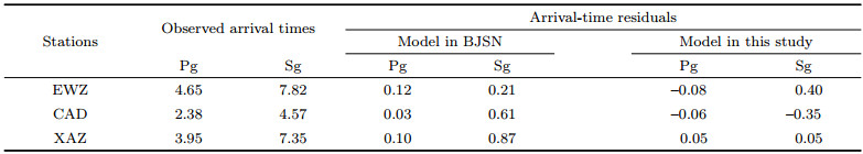
The 3-D crustal velocity structure beneath North China has been investigated intensely by seismologists such as Jia et al. (2005), Qi et al. (2006) and Yu et al. (2010). Their investigations reveal that the lateral heterogeneity along the line AB is weak. Besides, one-dimensional models are widely used in modern seismic networks for locating earthquakes. Therefore, we also employ a 1-D model, which consists of three layers. The thicknesses (H) and velocities of P (vP) and S (vS) waves of these layers from top to bottom are: H1=5 km, vP1=5.0 km·s−1, vS1=2.6 km·s−1; H2=15 km, vP2=6.1 km·s−1, vS2=3.5 km·s−1; H3=15 km, vP3=6.8 km·s−1, and vS3=3.9 km·s−1. The construction of the model is based on the observed traveltimes and by reference to a model of eastern North China (Teng et al, 1979). We divide the model into 0.1 km×0.1 km square elements. For the hypocenter determined by BJSN, the travel-time residuals with respect to our model are shown in Table 2. These residuals suggest our constructed model is acceptable.
4.2.2 Hypocentral lociStations EWZ, CAD and XAZ are combined into pairs. In this way, there are three P-wave arrival time difference constrained hypocentral loci as shown in Fig. 7a. Different loci are drawn in different colors. As can be seen, these loci are approximately similar to hyperbolas, and intersect at one point slightly to the right and below the hypocenter (the red “+”) located by BJSN. Fig. 7b shows the hypocentral loci constrained with arrival time differences between P and S waves at the same stations. The red, green and blue lines respectively correspond to the three stations in left-to-right order. These lines are basically circular in despite of the vertical heterogeneity. Their intersection points spread out. Noticeably, the locus to station EWZ (the red) runs away from the hypocentral location given by BJSN. That is probably related to the large travel time residual of Sg phase at this station. As for the phenomenon that the loci to stations EWZ and XAZ have gaps at the first interface, it results from the fact that seismic waves from the two stations are refracted and travel along the interface, and consequently their travel times change sharply at the refraction interface.

|
Fig. 7 Hypocentral loci of the real event (a) Constraint of arrival time differences between P waves; (b) Constraint of those between P and S waves; (c) Constraint of P-wave arrival times; (d) Constraint of P-and S-wave ones. The red signs of “+” indicate the hypocenter located by Beijing seismic network. |
The hypocentral loci constrained with P-wave arrival times are shown in Fig. 7c. The red, green and blue lines respectively correspond to stations EWZ, CAD and XAZ. Among these loci, two are similar to hyperbolas and one near to be circular. The three loci not only intersect at one point but also have a good directional distribution. Especially they impose a tight constraint upon the hypocentral depth. Thus, we infer that the actual hypocenter is somewhat deeper than and to the northeast of that by BJSN. Fig. 7d shows the hypocentral loci constrained with both P-and S-wave arrivals. The red, green and blue lines respectively correspond to stations EWZ, CAD and XAZ; the solid and dashed lines correspond to P and S waves, respectively. Similar to Fig. 7b, the loci in Fig. 7d do not intersect at one point either. However, their intersection area contains the hypocenter located by BJSN. Why hypocentral loci constrained with both P-and S-waves intersect sparsely, different from those with alone P-waves, is perhaps that there are large errors in the picked arrivals or/and the velocities of S waves.
5 DISCUSSIONS 5.1 Stability of Hypocentral LociThe calculation results of the complex model show that in the view of the directional distribution of hypocentral loci, far stations sometimes seem more adequate for constraining the hypocentral depth (see Fig. 4a and Fig. 5i). That directly contradicts with the common sense. Actually, as for hypocentral loci of an event, how tightly they constrain the hypocenter depends on their stability as well as their directional distribution near the source. When the residual field is regarded as a topographic map, the hypocentral locus in it accordingly lies in a valley. The steeper the valley is, the stabler the locus is; the gentler the valley is, the unstabler the locus is.
Figure 8a presents the arrival time residual field of the hypocentral locus marked with a red circle in Fig. 5a, which corresponds to station R6. It is noticeable that the locus has two (left and right) segments. Compared with the left part, the low residual (for example, smaller than 0.1 s) zone containing the right segment is rather wide, thereby the latter is decidedly less stable. The blue lines express the calculated hypocentral locus for RFLRP=0.01 s. By comparison with Fig. 5a, the new calculation result is slightly different and better represents the truth at the part marked with the red circle. When the observations are disturbed by random noise, the right segment with weak stability changes dramatically, as is shown by the part in Fig. 5k marked with the red circle; whereas the right one changes slightly because of its strong stability. This means that unstable hypocentral loci are easily influenced by disturbances.

|
Fig. 8 Hypocentral loci in the fields of RAT (residual of arrival time) for the event in the complex model (a) The hypocentral locus is constrained with the P wave arrival time at station R6, and its origin time field is constructed with P-wave data from all the nine stations. (b) and (c) The hypocentral loci are constrained with the same P-wave arrival time at station R9, but their origin time fields are constructed with only P-wave, and both P-and S-wave data from stations R7 − R9, respectively. The red “+” indicate the true hypocenter. |
For the sake of more clearly illustrating the actual role of far stations in constraining the hypocentral depth, we take into account the hypocentral loci constrained with arrival times at stations R7, R8 and R9. Fig. 8b shows the locus for P-wave arrival at station R9 and its arrival time residual field when the origin time field is constructed with P-wave data alone. Although the locus extends almost in the horizontal direction near the source, it can not tightly constrain the hypocentral depth because its stability is rather weak, especially in the vicinity of the hypocenter; accordingly, it is probably changed significantly in position and shape even by small disturbances. When the S-wave arrival times are additionally used in the construction of the origin time field, the resultant locus corresponding to the same arrival is much stabler, as Fig. 8c shows. This case is similar to those of the loci corresponding to stations R7 and R8. By this token, the effect of additionally using S-wave arrival times on the strengthening of the constraint on the hypocentral location is reflected in the improvement not only in the directional distribution of hypocentral loci, but also in their stability.
5.2 Selection of the Calculation Parameters for Hypocentral LociThe parameter RFLRP for selecting HLRPs controls the number of primary HLRPs. To ensure the intactness of the locus, the primary HLRPs are required to include the nodes of the model elements where individual endpoints of all the locus segments exist. In other words, the maximum of the residuals at the endpoints is the lower limit of RFLRP. The lower limit usually increases with increasing element size and decreasing seismic velocity. On the other hand, for we repeatedly “peel off” the skin of the set of primary HLRPs to retain its core as the final HLRPs, RFLRP must not be so large that the resultant primary HLRPs form connected regions with more than one core. Namely, it is desirable that each connected region contains only one locus segment. Actually, RFLRP has a quite wide range of values meeting the above requirements. Fig. 9 shows the variation of the percentages of primary (dashed line) and final (solid line) HLRPs in the total model nodes with increasing RFLRP for the P-wave arrival time constrained hypocentral locus in the homogeneous model. The step of RFLRP is taken to be 0.005 s. As can be seen, the number of the final HLRPs changes very little when RFLRP varies within a fairly wide range from about 0.03 s to 0.5 s. This stability suggests that the parameter RFLRP does not need adjusting with the geometry of hypocentral loci, which is beneficial to the automated processing of large batches of data. The value of RFLRP, under the condition that the calculated locus is complete, is suggested to be as small as possible. This not only saves computational time but also ensures good representativeness of the selected HLRPs for weakly stable hypocentral loci.

|
Fig. 9 Percentages of primary (dashed line) and final (solid line) reference points for the focal locus in Fig. 1c |
The parameter RFL associated with the calculation of ray paths controls the ray tracing area. To ensure the intactness of the hypocentral locus and prevent false hypocentral loci, the connected regions with residuals less than RFL are required that they each completely contain one and only one locus segment. Namely, RFL must be no less than the maximum of residuals at the model nodes crossed by the hypocentral locus but must not be so large that there is one or more connected region with more than one locus segment. When the hypocentral locus is one-segmented, the upper limit of RFL can be large enough that the ray tracing area extends to the whole model space. As for a multi-segment hypocentral locus, the value range of RFL is fairly wide. Taking Fig. 8a as an example, it is proper to choose RFL within the range of 0.1~0.5 s. For a small value of RFL, the ray tracing area is one or more narrow zones of which the percentage in the model region is very low, and accordingly the calculation of the hypocentral locus is fast.
The modification parameter Ltwig of hypocentral loci controls the length of ray paths to be removed. Its value is related to the selected HLRPs. When HLRPs are distributed along the hypocentral locus, resulting in short ray paths without branching, the value of Ltwig can be chosen relatively small. When the hypocentral locus is weakly stable and the parameter RFLRP is rather large, the final HLRPs probably contain poorly representative points. In this case, Ltwig should be chosen a large value so as to remove the rays to the points away from the hypocentral locus.
5.3 Extension of the Algorithm to Three DimensionsEarthquake location is a three-dimensional problem. In a three-dimensional residual field, nodes of the model elements crossed by the hypocentral locus are local minimum points. These nodes lie in the middle of the low residual regions, and are more similar to one or more cores of a fruit. Therefore, the peeling algorithm for selecting HLRPs is adapted to three dimensions except for slight difference in the elimination of superfluous HLRPs. As for ray paths, they are calculated with the minimum traveltime tree algorithm which has the same frame for two-and three-dimensional models. In the case of three dimensions, the calculated ray paths also form tree structures, and hence they can be modified to be finer in the similar way to that of trimming branches. Thus, the improved method presented in this study can be easily extended to three-dimensional models by means of 3-D minimum traveltime tree algorithms (Klimeš et al., 1994; Wang et al., 2000; Zhao et al., 2004). Compared with two-dimensional models, the calculation of hypocentral loci in 3-D models costs much more computational time, mainly because it is time consuming to model the three-dimensional travel time fields that shot points are located at stations. However, the time consuming step is needed only once. Therefore, the method is quite efficient in calculating hypocentral loci of numerous events within a region that has a stable velocity structure, recorded by the same seismic network.
6 CONCLUSIONSThe improved method put forward in this article for calculating hypocentral loci is as robust as the original one and hence suitable for complex models. Moreover, it works well in maintaining the completeness and the fineness of calculated hypocentral loci. There are no restrictions on the number of segments that constitute a hypocentral locus. The ray tracing is confined to low residual regions, and that saves a large amount of calculation time. The parameters for calculating hypocentral loci are easy to choose and do not need to be adjusted frequently with geometry of the loci. This is favorable for the automated processing of large batches of data. Additionally, the improved method can be easily extended to three dimensions. Its calculation efficiency is quite high for more than one event from a region with a stable velocity structure, recorded by the same seismic stations because the most time consuming travel time calculations have to be done only once.
The numerical tests indicate that hypocentral loci constrained with arrival time differences are different in form from those with arrival times, and the latter are quite complex even for homogeneous media. The capability of focal loci to constrain the hypocenter depends on their directional distribution near the source and their stability. Arrival times at near stations are strong in constraining the hypocentral depth. When both the velocity model and the picked arrival times are fairly accurate, the additional use of S-wave data can significantly improve the constraint upon the hypocentral location, especially for events outside the seismic network. Using more hypocentral loci can decrease the influence of random factors on earthquake location.
ACKNOWLEDGMENTSThis work is supported by the National Natural Science Foundation of China (41374098 and 40974050) and the Special Foundation for Basic Professional Scientific Research (DQJB11C03). We thank Professor
| [] | Bai L, Zhang T Z, Zhang H Z. 2003. Multiplet relative location and wave correlation correction and their application. Acta Seismologica Sinica (in Chinese) , 25 (6) : 591-600. |
| [] | Bai Z M, Wang C Y. 2003. Tomographic investigation of the upper crustal structure and seismotectonic environments in Yunnan Province. Acta Seismologica Sinica (in Chinese) , 25 (2) : 117-127. |
| [] | Bai Z M, Wang C Y. 2004. Tomography research of the Zhefang-Binchuan and Menglian-Malong wide-angle seismic profiles in Yunnan province. Chinese J. Geophys. (in Chinese) , 47 (2) : 257-267. |
| [] | Billings S D, Sambridge M S, Kennett B L N. 1994. Errors in hypocenter location:picking, model, and magnitude dependence. Bull. Seism. Soc. Am. , 84 (6) : 1978-1990. |
| [] | Bondár I, Myers S C, Engdahl E R, et al. 2004. Epicentre accuracy based on seismic network criteria. Geophys. J. Int. , 156 (3) : 483-496. DOI:10.1111/gji.2004.156.issue-3 |
| [] | Cai M J, Shan X M, Xu Y, et al. 2004. Review of earthquake-locating methods from error. Journal of Seismological Research (in Chinese) , 27 (4) : 314-317. |
| [] | Cao S H, Greenhalgh S. 1993. Calculation of the seismic first-break time field and its ray path distribution using a minimum traveltime tree algorithm. Geophys. J. Int. , 114 (3) : 593-600. DOI:10.1111/gji.1993.114.issue-3 |
| [] | Chen H, Chiu J M, Pujol J, et al. 2006. A simple algorithm for local earthquake location using 3D VP and VS Models:test examples in the central United States and in central eastern Taiwan. Bull. Seismol. Soc. Am. , 96 (1) : 288-305. DOI:10.1785/0120040102 |
| [] | Chen Y T. 2009. Earthquake prediction:Retrospect and prospect. Sci. China Ser. D-Earth Sci. (in Chinese) , 39 (12) : 1633-1658. |
| [] | Ding Z F, He Z Q, Sun W G, et al. 1999. 3-D crust and upper mantle velocity structure in eastern Tibetan plateau and its surrounding areas. Chinese J. Geophys. (in Chinese) , 42 (2) : 197-205. |
| [] | Font Y, Kao H, Lallemand S, et al. 2004. Hypocentre determination offshore of eastern Taiwan using the Maximum Intersection method. Geophys. J. Int. , 158 : 655-675. DOI:10.1111/gji.2004.158.issue-2 |
| [] | Geiger L. 1912. Probability method for the determination of earthquake epicenters from the arrival time only. Bull. St. Louis Univ. , 8 : 60-71. |
| [] | Jia S X, Qi C, Wang F Y, et al. 2005. Three-dimensional crustal gridded structure of the Capital area. Chinese J. Geophys. (in Chinese) , 48 (6) : 1316-1324. DOI:10.1002/cjg2.779 |
| [] | Jiang C S, Wu Z L, Li Y T. 2008. Estimating the location accuracy of the Beijing Capital Digital Seismograph Network using repeating events. Chinese J. Geophys. (in Chinese) , 51 (3) : 817-827. |
| [] | Kan R J, Hu H X, Zeng R S, et al. 1986. Crustal structure of Yunnan province, People's Republic of China, from seismic refraction profiles. Science , 234 (4775) : 433-437. DOI:10.1126/science.234.4775.433 |
| [] | Klimeš L, Kvasnika M. 1994. 3-D network ray tracing. Geophys. J. Int. , 116 (3) : 726-738. DOI:10.1111/gji.1994.116.issue-3 |
| [] | Lian C, Li S L, Dong M, et al. 2006. Method of spherical surface shearing in earthquake location. Journal of Geodesy and Geodynamics (in Chinese) , 26 (2) : 99-103. |
| [] | Meng Y M, Zhao Y, Wang B. 2001. The analysis on deviation of rapid location by China Seismic observational Network. Earthquake (in Chinese) , 21 (3) : 65-69. |
| [] | Moser T J. 1991. Shortest path calculation of seismic rays. Geophysics , 56 (1) : 59-67. DOI:10.1190/1.1442958 |
| [] | Nakanishi I, Yamaguchi K. 1986. A numerical experiment on nonlinear image reconstruction from first-arrival times for two-dimensional island arc structure. J. Phys. Earth , 34 (2) : 195-201. DOI:10.4294/jpe1952.34.195 |
| [] | Pujol J. 2004. Earthquake location tutorial:graphical approach and approximate epicentral location techniques. Seismol. Res. Lett. , 75 (1) : 63-74. DOI:10.1785/gssrl.75.1.63 |
| [] | Qi C, Zhao D P, Chen Y, et al. 2006. 3-D P and S wave velocity structures and their relationship to strong earthquakes in the Chinese capital region. Chinese J. Geophys. (in Chinese) , 49 (3) : 805-815. |
| [] | Richards P G, Waldhauser F, Schaff D, et al. 2006. The applicability of modern methods of earthquake location. Pure and Applied Geophysics , 163 (2-3) : 351-372. DOI:10.1007/s00024-005-0019-5 |
| [] | Shearer P M. 1997. Improving local earthquake locations using the L1 norm and waveform cross correlation:Application to the Whittier Narrows, California, aftershock sequence. J. Geophys. Res. , 102 (B4) : 8269-8283. DOI:10.1029/96JB03228 |
| [] | Song R, Gu X H, Wang Y L, et al. 2001. The software system for real-time processing and large earthquake rapid determination of NCDSN. Earthquake (in Chinese) , 21 (4) : 47-59. |
| [] | Teng J W, Yao H, Zhou H N. 1979. Crustal structure in the Beijing-Tianjin-Tangshan-Zhangjiakou region. Acta Geophysica Sinica (in Chinese) , 22 (3) : 218-236. |
| [] | Teng J W, Zhang Z J, Zhang X K, et al. 2013. Investigation of the Moho discontinuity beneath the Chinese mainland using deep seismic sounding profiles. Tectonophysics , 609 : 202-216. DOI:10.1016/j.tecto.2012.11.024 |
| [] | Theunissen T, Font Y, Lallemand S, et al. 2012. Improvements of the Maximum Intersection Method for 3D Absolute Earthquake Locations. Bull. Seismol. Soc. Am. , 102 (4) : 1764-1785. DOI:10.1785/0120100311 |
| [] | Tian Y, Chen X F. 2002. Review of seismic location study. Progress in Geophysics (in Chinese) , 17 (1) : 147-155. |
| [] | UdÍas A. 1999. Principles of Seismology[M]. Cambridge: Cambridge University Press . |
| [] | Waldhauser F, Ellsworth W L. 2000. A double-difference earthquake location algorithm:method and application to the northern Hayward fault, California. Bull. Seismol. Soc. Am. , 90 (6) : 1353-1368. DOI:10.1785/0120000006 |
| [] | Wang C Y, Mooney W D, Wang X L, et al. 2002. Study on 3-D velocity structure of crust and upper mantle in Sichuan-Yunnan Region, China. Acta Seismologica Sinica (in Chinese) , 24 (1) : 1-16. |
| [] | Wang H, Chang X. 2000. 3-D ray tracing method based on graphic structure. Chinese J. Geophys. (in Chinese) , 43 (4) : 534-541. |
| [] | Xu L S, Du H L, Yan C, et al. 2013a. A method for determination of earthquake hypocentroid:time-reversal imaging technique I-Principle and numerical tests. Chinese J. Geophys. (in Chinese) , 56 (4) : 1190-1206. DOI:10.6038/cjg20130414 |
| [] | Xu L S, Yan C, Zhang X, et al. 2013b. A method for determination of earthquake hypocentroid:time-reversal imaging technique II-An examination based on people-made earthquakes. Chinese J. Geophys. (in Chinese) , 56 (12) : 4009-4027. DOI:10.6038/cjg20131207 |
| [] | Yang W D, Jin X, Li S Y, et al. 2005. Study of seismic location methods. Earthquake Engineering and Engineering Vibration (in Chinese) , 25 (1) : 14-20. |
| [] | Yu X W, Chen Y T, Zhang H. 2010. Three-dimensional crustal P-wave velocity structure and seismicity analysis in Beijing-Tianjin-Tangshan Region. Chinese J. Geophys. (in Chinese) , 53 (8) : 1817-1828. DOI:10.3969/j.issn.0001-5733.2010.08.007 |
| [] | Zeng R S. 1991. The problems of lithospheric structure and geodynamics. Advance in Earth Sciences (in Chinese) , 6 (2) : 1-10. |
| [] | Zhang Z J, Yang L Q, Teng J W, et al. 2011. An overview of the earth crust under China. Earth-Science Reviews , 104 (1-3) : 143-166. DOI:10.1016/j.earscirev.2010.10.003 |
| [] | Zhao A H, Zhang Z J, Peng S P. 2003. Fast ray tracing method for converted waves in complex media. Journal of China University of Mining & Technology (in Chinese) , 32 (5) : 513-516. |
| [] | Zhao A H, Zhang Z J. 2004. Fast calculation of converted wave traveltime in 3-D complex media. Chinese J. Geophys.(in Chinese) , 47 (4) : 702-707. |
| [] | Zhao A H, Zhang Z J, Teng J W. 2004. Minimum travel time tree algorithm for seismic ray tracing:improvement in efficiency. J. Geophy. Eng. , 1 (4) : 245-251. DOI:10.1088/1742-2132/1/4/001 |
| [] | Zhao A H, Ding Z F. 2007. An intersection method for locating earthquakes in complex velocity models. Applied Geophysics , 4 (4) : 294-300. DOI:10.1007/s11770-007-0036-5 |
| [] | Zhao A H, Ding Z F, Sun W G, et al. 2008. Calculation of focal loci for earthquake location in complex media. Chinese J. Geophys. (in Chinese) , 51 (4) : 1188-1195. |
| [] | Zhao A H, Ding Z F. 2009. Earthquake location in transversely isotropic media with a tilted symmetry axis. J. Seismol. , 13 (2) : 301-311. DOI:10.1007/s10950-008-9129-8 |
| [] | Zhao A H. 2104. Hypocentral loci in earthquake location under the constraint of arrival time residual norm.//Chen Y T, Jin Z M, Shi Y L, et al. A Study of Interior Physics and Dynamics of Continental China-in Honor of Academician Teng Jiwen's 60th Anniversary of being Engaged in Geophysical Research (in Chinese). Beijing:Science Press, 265-280. |
| [] | Zhou H W. 1994. Rapid three-dimensional hypocentral determination using a master station method. J. Geophys. Res. , 99 (B8) : 15439-15455. DOI:10.1029/94JB00934 |
| [] | Zhou J C, Zhao A H. 2012. An intersection method for locating earthquakes in 3-D complex velocity models. Chinese J. Geophys. (in Chinese) , 55 (10) : 3347-3354. DOI:10.6038/j.issn.0001-5733.2012.10.017 |