 2015, Vol. 58


2 China University of Geosciences, State Key Laboratory of Geological Processes and Mineral Resources, Beijing 100083, China;
3 School of Geophysics and Information Technology, China University of Geosciences, Beijing 100083, China;
4 Center for Earthquake Research and Information, University of Memphis, Memphis 38152, USA
Topographic correction has been a great concern of geophysicists. It is one of the most heavy and important work in the data processing of gravity measurement. The theory and related practice of the physical geodesy show that the spatial distribution, movement and change of the Earth surface and interior matter determine the Earth’s gravity field and its change with time. Therefore, it is essential to accurately determine topographic relief.
In 1912, Hayford and Bowie, Hammer studied the influence of topography on gravity survey, put forward the topographic correction method that divides topography into sector partitions using concentric circles and radial lines, which is called circular domain method. With the application of computers Kane (1962) and others developed a series of methods which can be applied to computer calculation by digitizing terrain elevation data into square prism units and are called square domain method. No mass outside of the geoidal surface is the premise of applying Stokes formula, which requires that the influence of terrain mass outside of the geoidal surface to be removed (Moritz, 1980). Therefore, the research on local terrain correction is of great significance. By using the Gauss formula, Zhou and Li (1987) proposed the surface integration method of gravity terrain correction and obtained a simple formula to calculate gravity terrain correction with high precision. Liu and Xin (1992) regarded the Earth as an irregular rotation ellipsoid, divided the entire Earth with three spindle cone elements and presented an accurate calculation method of terrain correction. Calculating terrain correction using accurate polyhedron formula, the correction range can be arbitrary to the entire Earth.
An important part of the work of regional gravity is to apply the terrain information to the Earth’s gravity field, and get the terrain correction. Study of Wichiencharoen (1982), Bian and Zhang (1991), Lu (1989; 1996), Huang et al. (2000), Hofmann-Wellenhof and Moritz (2006), Zhang et al. (2006) show that the change of gravity value is determined by the removal and increase of terrain mass around the ground point. Bian proposed that the refinement of geoid must be supplemented by high resolution digital terrain model (Bian and Zhang, 1991). Many scholars have done some research on local terrain correction (Sideris, 1985; Schwarz et al., 1990; Sideris, 1990; Li, 1993; Sideris and Li, 1993; Novák et al., 2001; Xu, 2006). On the basis of existing problems, Guo and Xu (2011) proposed two methods to overcome the singularity of terrain correction formula, and derived the formula to deal with singular integrals using the Gauss integral method (Chou, 2005) and the strict series expansion of topographic correction with optional small constants. Conventionally, terrain is divided into Bouguer plate and local terrain. There are many kinds of plane approximate topographic correction methods, such as FFT spectrum method, prism integral method and cylinder integral method. In 1999, Novak divided terrain into Bouguer shell and rough terrain with Stokes-Helmert method and computed the direct and indirect effects of topography. There are obvious differences between the Bouguer spherical shell calculation formula and the Bouguer plate calculation formula (Novák et al., 2001). In 2001, Vanicek carried out an analysis of the above method, suggested that the calculation using Stokes-Helmert method and based on Bouguer shell is more reasonable (Vanicek et al., 2001).
Helmert condensation correction, isostatic correction and residual terrain model (RTM) are practical methods of terrain correction and calculation, among which Helmert condensation correction is used to correct the geoid, isostatic correction and residual terrain model (RTM) are used to correct height anomaly. Ning et al. (1996)’s experiment in a mountainous region showed that the influence of lateral inhomogeneous variation in the crustal density on surface gravity anomaly is several mGal, and its influence on the geoid can be centimeter level. Li and Liu (2003) showed in a study of classical Helmert correction, RTM and Helmert/RTM combination method that the fitting result of Helmert/RTM combination method and GPS/level data is the best. Wang (2011) performed physical stress analysis on the Earth surface and geoidal surface. The research found that traditional terrain correction methods produce errors, and presented the algorithm to improve the accuracy of terrain correction. Huang, Guo, Li and others have discussed the plane approximate terrain correction method (Guo et al., 2002; Li et al., 2003; Pang, 2008; Zhang, 2009; Guo, 2010; Zhang, 2012). Zhang believes that traditional planar Bouguer correction destroys the harmonic property of gravity field, which can only be used for surface gravity anomalies, and thus cannot be applied to other heights beyond the surface of the Earth (Zhang et al., 2009; Zhang et al., 2012). Rong and Zhou (2015) introduced a division method which considers the geoid as a sphere, studied the terrain above the ground level, and compared the result with traditional plane approximations.
1.2 Topographic Correction in Geoelectric ProspectingIn gravity exploration, terrain is believed to be caused by the deficit and surplus of materials. Knowing the microscopic mechanism, terrain anomalies can be expressed as analytic formula. Different from gravity terrain correction, there is no such formula in geoelectric exploration. Specific relationship should be based on the analysis and summary of actual variation rules.
The observed values of geoelectric profile are influenced by topographies. There are three kinds of forms of geoelectric field interference caused by topography: the disappearance of the anomalies of the studied objects; the disappearance of some anomaly features of the research objects; the position movement of the anomalies of the studied objects. These phenomena often make the anomalies caused by research objects cannot be identified, or lead to wrong locations in the verification work. In addition, false anomalies may appear at locations where geological objects do not exist. With regard to the influence of topography on geoelectric profile method, theoretical calculations and model experiments have been carried out. Lin has carried out experimental work since 1963, simulated actual terrains with the soil troughs or thin troughs, corrected the observed values of the corresponding measurement points in the field using the observed values of the simulated terrains, and have obtained some results (Lin, 1966).
In order to make clear the influence of terrains on apparent resistivity method, model experiments and theoretical calculations have been carried out. Xu (1966) derived and calculated the plane parallel electric field curves of finite length valleys and ridges, and the line source field current density curves of some simple smooth terrain. Maeda (1955) did some research on the formula of point source field potential in infinite long ridges and valleys. Ge (1977) proposed a theoretical calculation method to eliminate the influence of complex terrain on apparent resistivity. Huang (1986) verified the correctness of apparent resistivity numerical solutions of angular domain topographies by analytical method. The practice showed that the apparent resistivity curves of terrain correction by using boundary element method make the anomalies of target objects significant; and the boundary element method of 2-D terrain correction by point source field resistivity method is an economical and effective method.
Theoretical research and a large number of field practices have fully demonstrated that terrain correction with the method of comparison can weaken terrain interferences and make the useful anomalies significant, so it can effectively improve the geological effects of geoelectric prospecting (He and Zeng, 1984). There are two kinds of methods to obtain pure terrain anomalies: use conformal mapping or thin water layer model experiment and two-dimensional resistance network to obtain curves of 2D terrains; and calculate using the analytical formula of pure topographic potentials, or obtain point source 2D or 3D terrain anomaly curves using physical simulation and numerical simulation (such as the finite element method).
Xu (1985), Wannamaker et al. (1986), Chouteau and Bouchard (1988) have used the finite element method to study the influence of two dimensional terrains on the Earth’s electromagnetic field. The research showed that Hx waves are significantly affected by two dimensional terrains, while Ex waves are less affected. Xu (1995) studied the same problem by using boundary element method, and drew the same conclusion. On the basis of this, Xu et al. (1997) simplified the calculation method of the influence of two dimensional terrain on Hx waves. The experimental results showed that boundary element method is effective for 2-D terrain correction of Hx waves.
The terrain influence on Mise-A-LA-Masse method comes from two factors (He and Xia, 1978): first, the distribution of underground electric field is changed by topography fluctuation; second, the distance between the measuring point and the field source is changed in the undulating terrain. He and Xia (1978), Fu (1983) discussed a variety of topographic correction methods to eliminate the influence of topography. Dai and Luo (1997) discussed the problems existing in methods of topographic correction of Mise-A-LA-Masse method, and proposed a terrain correction method based on ratio method.
2 TERRAIN CORRECTION IN THE GRADIENT CALCULATION OF SPONTANEOUS POTENTIAL DATAAt present, there are no other authors who have studied the terrain correction in the gradient calculation of spontaneous potential data. According to research by the author of this paper, terrain relief can influence the appearance of anomalies, especially when the area of rugged terrain is comparable to the area of geological bodies, in which case it is difficult to distinguish these two anomalies. Topographic correction is essential (Wang et al., 2000; Wang et al., 2003; Li et al., 2005).
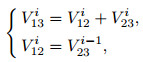
2.1 Method of Gradient CalculationDuring field work, the height Ai and potential differences V12i, V13i and V23i should be recorded synchronously. Data recorded should satisfy in theory
|
(1) |
where V is the potential difference between two points in unit mV. Each V23 should be approximately equal to the next V12 with an error of 1 mV allowed.
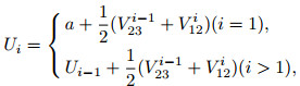
Because the observations are potential differences between every two points, they cannot reflect underground situations, and thus need to be transformed into potential. The specific treatment method is as follows:
|
(2) |
where Ui is the spontaneous potential after superposition in unit mV; a is the spontaneous potential at the starting point of the measuring line. It can be set to 0 mV or a particular value.
After processing by Eq.(2), the average values of V23 and V12 corresponding to the measured data will be used as the potential differences between measuring points. The potential differences will be then superimposed to obtain the spontaneous potential of each point. When doing corrections, the sequence of “contrast correction→data superposition→diurnal correction→terrain correction” should be followed. First, the effect of electrode contrasts should be eliminated, and then the measured data should be superimposed so that the potential differences will be converted to potential, then the influence of diurnal variation should be eliminated, and finally the topographic correction should be done on the basis of contrast correction and diurnal correction.
2.2 Principle of Terrain CorrectionAs shown in Fig. 1, in the gradient calculation of spontaneous potential data, terrain anomalies are divided into two types: one is that anomalies and topographies are mirror image relation, this kind of situation occupies the majority; another kind of situation is that anomalies and topographies are inverse mirror image relation, which is rarely seen in oil and gas exploration (Junheng et al., 2007; Wang et al., 2007). There are three kinds of relationship between terrain fluctuations and anomalies: linear, quadratic, or exponential, which can be used for correction. The relationships are

|
Fig. 1 The potential caused by topography |
|
(3) |
|
(4) |
|
(5) |
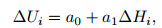
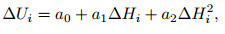
where ∆Ui is the potential correction value in unit mV; ∆Hi is the relative elevation in unit m; a0, a1, a2, A, B, C are dimensionless constant coefficients. The specific relationship should be decided according to the observation of actual variation rules. A small number of terrains have complex relationship with anomalies, and can be corrected with the method of relevant analysis.
When the data is processed, the spontaneous potential of the points where elevations are recorded can be obtained. When doing the correction, the relative height curve and spontaneous potential curve of each line should be plotted first. A section of large undulating terrain should be selected from the relative height curve, and its corresponding spontaneous potential could be found through measuring points. So, a set of relative height {∆H1, ∆H2, ∆H3, …, ∆Hn} and the corresponding spontaneous potential {∆U1, ∆U2, ∆U3, …, ∆Un} can be obtained, where n is the number of the fitting data.
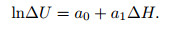
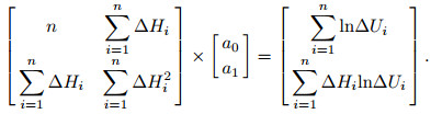
If spontaneous potential is assumed to be a linear function of relative elevation, i.e. ∆U=f(∆H)=a0 + a1∆H, the least square fitting formula
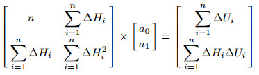
|
(6) |
can be applied to obtain the values of coefficient a0 and a1, thus the linear fitting formula of spontaneous potential correction amount about relative elevation Eq.(3) can be obtained.
If spontaneous potential is assumed to be a quadratic function of relative elevation, i.e. ∆U=f(∆H)=a0 + a1∆H + a2∆H2, the least square fitting formula
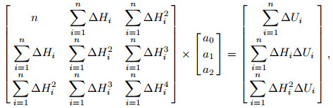
|
(7) |
can be applied to obtain the values of coefficient a0, a1 and a2, and thus the quadratic fitting formula of spontaneous potential correction amount about relative elevation Eq.(4) can be obtained.
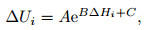
If spontaneous potential is assumed to be an exponential function of relative elevation, i.e. ∆U=f(∆H)=AeB∆H+C, then logarithm can be performed on both sides of the equation first, which gives
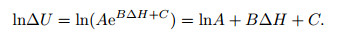
|
(8) |
Because lnA and C can be combined into one constant, let lnA=a0, B=a1, C=0, so
|
(9) |
Thus the exponent function is transformed into linear function, and then the derivation of least square formula of linear regression fitting can be referred to get
|
(10) |
The values of constant a0 and a1 can be calculated through the formula, and with the use of A=ea0, B=a1, C=0, the exponential fitting formula of spontaneous potential correction amount about relative elevation Eq.(5) can be obtained. Eqs.(3), (4) and (5) can be used to calculate the spontaneous potential correction amount of each measuring point, and then the spontaneous potential curves can be corrected through this terrain correction amount.
3 THE TOPOGRAPHIC CORRECTION IN ORDOS BASIN 3.1 Project OverviewThe work area belongs to a loess plateau in which there are several large residual loess platforms. The rest had been washed and cut into dendritic. Cretaceous is exposed in big ditches, and Tertiary lateritic or Quaternary loess layers are found in branch channels. The total thickness of loess layer and laterite is about 100 to 150 meters. Gullies, hills, ridges and plateaus are arranged in crisscross patterns with relative height of up to 250~300 m. Slopes are steep and regular in shape, which is one of the best places to study terrain correction in China. Five measuring lines were deployed in east-west direction and seven measuring lines were deployed in north-south direction, respectively.
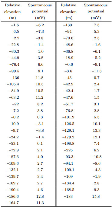
3.2 The Selection of Fitting DataThe fitting data used for topographic correction need to be selected following the following principles: (1) Large undulating terrains; (2) The spontaneous potential anomalies induced by terrains are very obvious; (3) Good corresponding relationship exists between topographies and anomalies. Line N1 is a line with large undulating terrains. It ran approximately in the north-south direction and went through two depression zones. 1300 m was set as the average elevation of this area. A chunk of data with large elevation variations was selected to plot the relative height curve and the spontaneous potential curve, as shown in Fig. 2.

|
Fig. 2 The mirror image relationship between the relative height curve and the spontaneous potential curve of the large undulating terrain section of N1 |
It can be seen that undulating terrains caused significant spontaneous potential changes, which caused large disturbance to the reflection of underground geological information. Generally mirroring relationship between the two is shown. A decrease of terrain by 200 m caused a positive anomaly of spontaneous potential by about 15 mV. The terrain slope reached maximum at measuring points 310 to 326, 340 to 352, 374 to 392 and 400 to 418, and the corresponding spontaneous potential anomalies are the most obvious, and thus can be used as the least squares fitting data. After using the same method to select some fitting data from several other measuring lines, a series of relative elevation and the corresponding spontaneous potential were obtained, as shown in Table 1.
|
|
Table 1 The relative height and their corresponding spontaneous potential that are used for fitting |
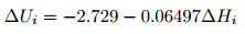
If it is assumed that the relative height and the spontaneous potential meet a linear function relation, the parameters values of a0=−2.729, a1=−0.06497 can then be calculated using the least square fitting formula (6), and the linear fitting formula between spontaneous potential correction amount and relative height,
|
(11) |
can thus be obtained.
If it is assumed that the relative height and the spontaneous potential meet a quadratic function relation, the parameters values of a0=−3.901, a1=−0.1099 and a2=−0.0002387 can then be calculated using the least square fitting formula (7), and the quadratic fitting formula between spontaneous potential correction amount and relative height,

|
(12) |
can thus be obtained.
If it is assumed that the relative height and the spontaneous potential meet an exponential function relation, the parameters values of a0=−0.08927, a1=−0.01193, i.e. A=0.9146, B=−0.01193, C=0 can then be calculated using the least square fitting Eq.(10), and the exponential fitting formula between spontaneous potential correction amount and relative height,
|
(13) |
can thus be obtained. The fitting curves are shown in Fig. 3.

|
Fig. 3 The linear fitting, quadratic fitting and exponential fitting curves implemented by applying the least squares formula (6), (7) and (10) |
It can be seen from the curves that the quadratic term coefficient a2 in the quadratic fitting formula (12) is very small, so the quadratic fitting curve and linear fitting curve are very close. The exponential fitting curve is close to the linear fitting curve in the relative elevation interval (–200 m, –50 m); when the relative elevation is above –50 m, the terrain correction amount of the exponential fitting formula is close to zero. A curve section of line N5 with large undulating terrains was taken as an example to analyze and compare the correction effects of three different fitting formulas. The relative elevation after measuring point 250 is about –250 m. The linear, quadratic and exponential fitting formula (11), (12) and (13) have been used to correct the measuring line respectively. The correction results are shown in Fig. 4.

|
Fig. 4 The spontaneous potential curves of the large undulating terrain section of N5 before and after topography correction by applying the linear fitting formula, the quadratic fitting formula and the exponential fitting formula respectively (dashed line, the spontaneous potential curve before topography correction; solid line is the spontaneous potential curve after topography correction) |
Seen from the above, affected by the falling of the terrain, the spontaneous potential curve of N5 after measuring point 250 was significantly raised up. No significant difference between the correction results of the three fitting formulas has been observed after measuring point 250; before measuring point 250, the correction result of the linear fitting formula is most remarkable, while almost no correction effect of the exponential fitting formula has been observed. This is because when the relative height is about –250 m, the fitting curves of the three formulas are very close (Fig. 3); when the relative height is greater than –50 m, the terrain correction amount of the exponential fitting formula is close to zero (Fig. 3). It thus can be seen that the linear fitting formula is a better way to describe the relationship between the topographic reliefs and the spontaneous potential in this section of the measuring line.
3.4 The Topographic Correction of the Surveyed AreaAfter all the 12 measuring lines (five in the eastwest and seven in the north-south) were processed with terrain correction, the relative height contour map of the surveyed area, the spontaneous potential contour map without terrain correction and the spontaneous potential contour map with terrain correction were plotted as in Figs. 5–7.

|
Fig. 5 The contour map of relative height in the surveyed area (measuring points were marked with black crosses) |

|
Fig. 6 The contour map of spontaneous potential after contrast correction and diurnal correction (measuring points were marked with black crosses) |

|
Fig. 7 The contour map of spontaneous potential after contrast correction, diurnal correction and topography correction (measuring points were marked with black crosses) |
It is seen from the figures that because of the great impact of the terrain of this region, the spontaneous potential flat contour map before terrain correction shows significant positive anomalies that are associated with concave terrains (marked with red rectangle in Fig. 6) and negative anomalies that are associated with raised terrains (marked with blue rectangle in Fig. 6). Terrain correction effectively eliminated the correlation between relative elevation and spontaneous potential, which made useful anomalies more prominent, and precluded the interference of underground geological information caused by terrain factors.
4 CONCLUSIONS(1) In the gradient calculation of spontaneous potential data, anomalies caused by topography were divided into two types: one is that anomalies have a mirror-image relation with terrain relief; the other one is that anomalies have an inverted mirror-image relation with terrain relief. The relation between a majority of anomalies and terrain relief could be linear, quadratic or exponential, which was used for fitting and correction.
(2) Because the mechanism of spontaneous potential anomalies formed by terrains is rather complex, it is difficult to obtain an analytic formula, whereas a more intuitive method can be adopted instead to find the fitting formula between these two variables. In this paper, the linear fitting formula, the quadratic fitting formula and the exponential fitting formula between relative elevation and spontaneous potential correction amount were proposed.
(3) Topographic correction in the gradient calculation of spontaneous potential data is realized by the method of calculating the coefficients of pre-assumed formulas. As for which fitting relation should be adopted specifically, it can be decided by selecting a typical terrain and spontaneous potential curve first and judging through the law of variations; and trial calculation method can be adopted as well to choose the appropriate fitting formula by comparing the correction effects. In this paper, the correction results of three fitting formulas were compared. It was then concluded that the linear fitting formula can better describe the relationship between the relative elevation and the spontaneous potential correction amount within this work area.
(4) The quality of terrain correction is evaluated by whether the correlation between terrain fluctuation and spontaneous potential was eliminated. Terrain correction is regarded to be effective when there is no significant mirror (or anti-mirror) relationship between terrain fluctuation and spontaneous potential.
| [] | Bian S F, Zhang K F. 1991. On the role of terrain in the refinement of the geoid in China. Progress in Geophysics (in Chinese) , 6 (4) : 64-74. |
| [] | Chouteau M, Bouchard K. 1988. Two-dimensional terrain correction in magnetotelluric surveys. Geophysics , 53 (6) : 854-862. DOI:10.1190/1.1442520 |
| [] | Dai G M, Luo T Z. 1997. A way of terrain correction for mise-a-la-masse method in 2 dimention. Computing Techniques for Geophysical and Geochemical Exploration (in Chinese) , 19 (1) : 36-40. |
| [] | Fu L K. 1983. Electrical Prospecting Tutorials (in Chinese)[M]. Beijing: Geological Publishing House . |
| [] | Ge W Z. 1977. Topographic correction for the DC apparent resistivity method of electrical prospecting. Acta Geophysica Sinica (in Chinese) , 20 (4) : 299-311. |
| [] | Gou C X, Wang H M, Wang B. 2002. Determination of high resolution grid terrain and isostatic corrections in all China area. Acta Geodaetica et Cartographica Sinica (in Chinese) , 31 (3) : 201-205. |
| [] | Guo D M. 2010. Refined theories, methods and applications of local quasi geoid[Ph. D. thesis] (in Chinese). Beijing:Graduate School of Chinese Academy of Sciences. |
| [] | Guo D M, Xu H Z. 2011. Research on the singular integral of local terrain correction computation. Chinese J. Geophys.(in Chinese) , 54 (4) : 977-983. DOI:10.3969/j.issn.0001-5733.2011.04.012 |
| [] | He J S, Zeng X M. 1984. Fast calculation using polynomes for topographic correction in resistivity method. Geophysical and Geochemical Exploration (in Chinese) , 8 (1) : 27-33. |
| [] | He Y S, Xia W F. 1978. The Excitation-at-the-Mass Method (in Chinese)[M]. Beijing: Geological Publishing House . |
| [] | Hofmann-Wellenhof B, Moritz H. 2006. Physical Geodesy. Wien:Springer Science & Business Media. |
| [] | Huang L Z, Tian X M, Cun S C. 1986. The boundary element method of the 2-D topographic correction for the resistivity method in the point source field. Computing Techniques for Geophysical and Geochemical Exploration (in Chinese) , 8 (3) : 201-208. |
| [] | Huang M T, Zhai G J, Guan Z, et al. 2000. On computations of terrain corrections and indirect effect using FFT. Journal of Institute of Surveying and Mapping (in Chinese) , 17 (4) : 242-246. |
| [] | Kane M F. 1962. A comprehensive system of terrain corrections using a digital computer. Geophysics , 27 (4) : 455-462. DOI:10.1190/1.1439044 |
| [] | Li J C, Chen J Y, Ning J S. 2003. The Approximation Theory of the Earth's Gravitational Field and the Determination of China 2000 Quasi-Geoid (in Chinese)[M]. Wuhan: Wuhan University Press . |
| [] | Li S S, Liu Y Y. 2003. Calculation of the reference orbit of CHAMP by gravitational potential model. Journal of Institute of Surveying and Mapping (in Chinese) , 20 (3) : 165-167. |
| [] | Li Y C. 1993. Optimized spectral geoid determination. UCSE Report No 20050. Calgary, Alberta, Canada:Geomatics Engineering, University of Calgary. |
| [] | Li Y L, Wang J H, Pan Z P, et al. 2005. Wavelet multiscale analysis and geophysical significance of the spontaneous potential of oil and gas reservoir. Petroleum Exploration and Development (in Chinese) , 32 (1) : 80-83. |
| [] | Lin C Y. 1966. The model experimental method of topographic correction in electric profiling method. Acta Geophysica Sinica (in Chinese) , 15 (1) : 66-72. |
| [] | Lin Z M, Shi Z S. 1984. A discussion on several terrain correction methods in regional gravity survey. Geophysical and Geochemical Exploration (in Chinese) , 8 (4) : 193-198. |
| [] | Liu L Y, Xin S C. 1992. A topographical correction method for gravity measurement based on a triangular polyhedron. Computing Techniques for Geophysical and Geochemical Exploration (in Chinese) , 14 (4) : 293-300. |
| [] | Lu Z L. 1989. Improving the Stokes solution of the disturbing potential with the help of topographic data. Acta Geodaetica et Cartographica Sinica (in Chinese) , 18 (1) : 60-71. |
| [] | Lu Z L. 1996. Theories and Methods of the Earth's Gravitational Field (in Chinese)[M]. Beijing: The People's Liberation Army Press . |
| [] | Maeda K. 1955. Apparent resistivity for dipping beds. Geophysics , 20 (1) : 123-139. DOI:10.1190/1.1438108 |
| [] | Ning J S, Luo Z C, Chao D B. 1996. The present situation on satellite gravity gradiometry and its vistas in the application of physical geodesy. Journal of Wuhan Technical University of Surveying and Mapping (in Chinese) , 21 (4) : 309-314. |
| [] | Novák P, VanÍek P, Martinec Z, et al. 2001. Effects of the spherical terrain on gravity and the geoid. Journal of Geodesy , 75 (9-10) : 491-504. DOI:10.1007/s001900100201 |
| [] | Pang Z X. 2008. Research on the refining methods of gravity anomaly[Master's thesis] (in Chinese). Zhengzhou:The PLA Information Engineering University. |
| [] | Rong M, Zhou W. 2015. Study on topography correction based on spherical approximation. Journal of Geodesy and Geodynamics (in Chinese) , 35 (1) : 58-61. |
| [] | Schwarz K P, Sideris M G, Forsberg R. 1990. The use of FFT techniques in physical geodesy. Geophysical Journal International , 100 (3) : 485-514. DOI:10.1111/gji.1990.100.issue-3 |
| [] | Sideris M G. 1985. A fast Fourier transform method for computing terrain corrections. Manuscripta Geodaetica , 10 (1) : 66-73. |
| [] | Sideris M G. 1990. Rigorous gravimetric terrain modelling using Molodensky's operator. Manuscripta Geodaetica , 15 (2) : 97-106. |
| [] | Sideris M G, Li Y C. 1993. Gravity field convolutions without windowing and edge effects. Bulletin Géodésique , 67 (2) : 107-118. DOI:10.1007/BF01371374 |
| [] | Vaniek P, Novák P, Martinec Z. 2001. Geoid, topography, and the Bouguer plate or shell. Journal of Geodesy , 75 (4) : 210-215. DOI:10.1007/s001900100165 |
| [] | Wang J H, Pan Z P, Guan Z N, et al. 2000. Self-potential detection principle of oil/gas reservoir and its application to field development. Petroleum Exploration and Development (in Chinese) , 27 (3) : 96-99. |
| [] | Wang J H, Pan Z P, Deng M S, et al. 2003. Relationship between spontaneous potential (SP) and apparent effective thickness (AET) of reservoirs. Petroleum Exploration and Development (in Chinese) , 30 (5) : 65-67. |
| [] | Wang J H, Pan Z P, Sun S W, et al. 2007. Apparent effective thickness prevision through spontaneous potential method and its application in oil development. Earth Science-Journal of China University of Geosciences (in Chinese) , 32 (4) : 461-468. |
| [] | Wang J H, Pan Z P, Sun S W, et al. 2007b. Prediction of apparent equivalent thickness using the spontaneous potential method and its application to oilfield development. Journal of China University of Geosciences , 18 (3) : 269-279. DOI:10.1016/S1002-0705(08)60007-2 |
| [] | Wang Z L, Wen L. 2011. A new terrain correction method. Journal of Geodesy and Geodynamics (in Chinese) , 31 (3) : 115-119. |
| [] | Wannamaker P E, Stodt J A, Rijo L. 1986. Two-dimensional topographic responses in magnetotellurics modeled using finite elements. Geophysics , 51 (11) : 2131-2144. DOI:10.1190/1.1442065 |
| [] | Wichiencharoen C. 1982. The indirect effects on the computation of geoid undulations. Report No. 336. Columbus, OH, United States:Dept. of Geodetic Science and Surveying, The Ohio State University. |
| [] | Xu H Z. 2006. Some problems on the precise determination of regional geoid in China. Geospatial Information (in Chinese) , 4 (5) : 1-3. |
| [] | Xu S Z. 1966. The impact of two-dimensional terrain on resistivity method. Acta Geophysica Sinica (in Chinese) , 15 (1) : 73-82. |
| [] | Xu S Z, Zhao S K. 1985. The topographic effects on magnetotelluric response. Northwestern Seismological Journal (in Chinese) , 7 (4) : 69-78. |
| [] | Xu S Z. 1995. The Boundary Element Method in Geophysics (in Chinese)[M]. Beijing: Science Press . |
| [] | Xu S Z, Li Y G, Liu B. 1997. The method and efficiency of 2-D terrain correction for HX-polarization of MT. Acta Geophysica Sinica (in Chinese) , 40 (6) : 842-846. |
| [] | Zhang C Y, Chao D B, Ding J, et al. 2006. Arithmetic and characters analysis of terrain effects for CM-order precision height anomaly. Acta Geodaetica et Cartographica Sinica (in Chinese) , 35 (4) : 308-314. |
| [] | Zhang C Y, Chao D B, Ding J, et al. 2009. Precision topographical effects for any kind of field quantities for any altitude. Acta Geodaetica et Cartographica Sinica (in Chinese) , 38 (1) : 28-34. |
| [] | Zhang C Y, Dang Y M, Ke B G, et al. 2012. Discussion of some lssues in the coastal precise quasi-geoid determination. Geomatics and Information Science of Wuhan University (in Chinese) , 37 (10) : 1150-1154. |
| [] | Zhou D Y. 2005. An innovation of 3-D non-singular boundary integral equations[Ph. D. thesis]. Taiwan:National Taiwan University. |
| [] | Zhou X X, Li X. 1987. Gravimetric terrain corrections by surface integration method. Computing Techniques for Geophysical and Geochemical Exploration (in Chinese) , 9 (4) : 273-279. |